6. Tools Overview

This section gives an overview over the additional tools contained in the FLEXI repository. It also lists the tutorials where they are used as reference. There are two different kinds of tools:

POSTI-tools can be compiled together with FLEXI given the according cmake options.
In the tools folder, a collection of shell and Python scripts can be found, which are mainly used to manage FLEXI runs and FLEXI output files.

6.1. POSTI Tools

The different POSTI tools are used to further post-process the simulation results obtained with FLEXI. They can be compiled together with FLEXI given the according cmake option. A list and description for the input parameters of the associated POSTI tools can be displayed with the command

[posti_toolname] --help

6.1.1. Visualization

6.1.1.1. POSTI_VISU

POSTI_VISU converts FLEXI StateFiles, TimeAverage, and BaseFlow files from the HDF5 format to the ParaView readable .vtu (single) or .pvtu (parallel) format.

The POSTI_VISU tool reads a separate parameter file as optional first argument, while the files to be visualized are passed as the last argument. Without specifying a separate parameter file, the parameters stored in the userblock of the files are used and only the conservative variables are visualized. The latter can be a single file or several files, specified either as simple space-separated list like Testcase_State_0.h5 Testcase_State_1.h5 or via standard wildcarding like Testcase_State_*.h5. The file must contain the entire volume solution, i.e., can be a StateFile or a TimeAverage file, for example.

For serial execution, the POSTI_VISU tool is invoked by entering

posti_visu [parameter_postiVisu.ini [parameter_flexi.ini]] <statefiles>

The tool also runs in parallel by prepending mpirun -np <no. processors> to the above command, as usual, provided the compiler option LIBS_USE_MPI is enabled.

mpirun -np <no. processors> posti_visu [parameter_postiVisu.ini [parameter_flexi.ini]] <statefiles>

Important

ParaView can only read state files up to $2\, GB$ in single mode (.vtu). Furthermore, the MPI-parallel HDF5 implementation internally uses a signed 32-bit integer, restricting the maximum chunk size to $2\, GB$ per thread. When post-processing with activated LIBS_USE_MPI flag, especially with large cases and large files as is often the case with TimeAverage files, the file size of approximately $2\, GB$ per core must not be exceeded. In this case, the number of cores used must be increased for MPI-parallel executable POSTI tools, or POSTI must be compiled with LIBS_USE_MPI=OFF.

The POSTI_VISU tool has a help function that describes the available parameters. This help can be invoked by running the tool with the flag --help

posti_visu --help

The most important runtime parameters to be set in parameter_postiVisu.ini are listed in the table below.

Table 6.1 POSTI_VISU parameters.
Parameter	Possible Values	Description
NodeTypeVisu	VISU / GAUSS / GAUSS-LOBATTO / VISU-INNER	Node type of visualization basis; the default VISU uses equidistant nodes which include the boundary points of the elements.
NVisu	1 / 2 / 3 / …	Polynomial degree used to sample the solution for visualization; if left unspecified, it defaults to using the number of collocation points per elements, i.e. $N+1$ per dimension. For high-quality visualization, it is usually advisable to choose a value higher than $N$ in order to keep interpolation errors small.
VarName	Density / VelocityX / …	Names of the variables to be visualized, parameter can be specified multiple times to visualize more than one variable and set to both conservatives (e.g. Density) and primitives (e.g. VelocityX). If left unspecified, it defaults to visualizing the five conservative variables.
BoundaryName	Density / WallFriction / y+ / …	Name of the boundary to visualize. Some variables can only be visualized on the boundary like WallFriction / y+.

In the following all available variables that can be used for visualization are listed.

Density, MomentumX, MomentumY, MomentumZ, EnergyStagnationDensity, VelocityX, VelocityY, VelocityZ, Pressure, Temperature, VelocityMagnitude, VelocitySound, Mach, EnergyStagnation  ,EnthalpyStagnation  ,Entropy  ,TotalTemperature  ,TotalPressure  ,PressureTimeDeriv  ,VorticityX  ,VorticityY  ,VorticityZ  ,VorticityMagnitude  ,NormalizedHelicity  ,Lambda2  ,Dilatation  ,QCriterion  ,Schlieren  ,WallFrictionX  ,WallFrictionY  ,WallFrictionZ  ,WallFrictionMagnitude  ,WallHeatTransfer  ,x+  ,y+  z+  

The practical application of POSTI_VISU is demonstrated in the following tutorials: Linear Scalar Advection-Diffusion Equation, Freestream, Lid-driven Cavity, SOD Shock Tube, Double Mach Reflection, Flow Around a Cylinder, Flow Around a NACA0012 Airfoil

6.1.1.2. ParaView Plugin

The FLEXI framework comes with a ParaView reader based on posti_visu to load the custom HDF5 state files directly into ParaView. It provides an interface to adjust the aforementioned posti_visu parameters in the ParaView GUI interactively. The plugin can be enabled through the compile flag POSTI_VISU_PARAVIEW=ON, but requires ParaView to be built from source.

In order to visualize the HDF5 state files, you need to load the compiled library build/lib/visuReader/visuReader.so via the ParaView menu Tools > Manage Plugins … > Load New …. Upon opening a FLEXI state file, this will show the Properties tab, as on the left in the screenshot below. The plugin allows you, for example, to modify parameters like NVisu, to select the variables for visualization and to display the imposed boundary conditions.

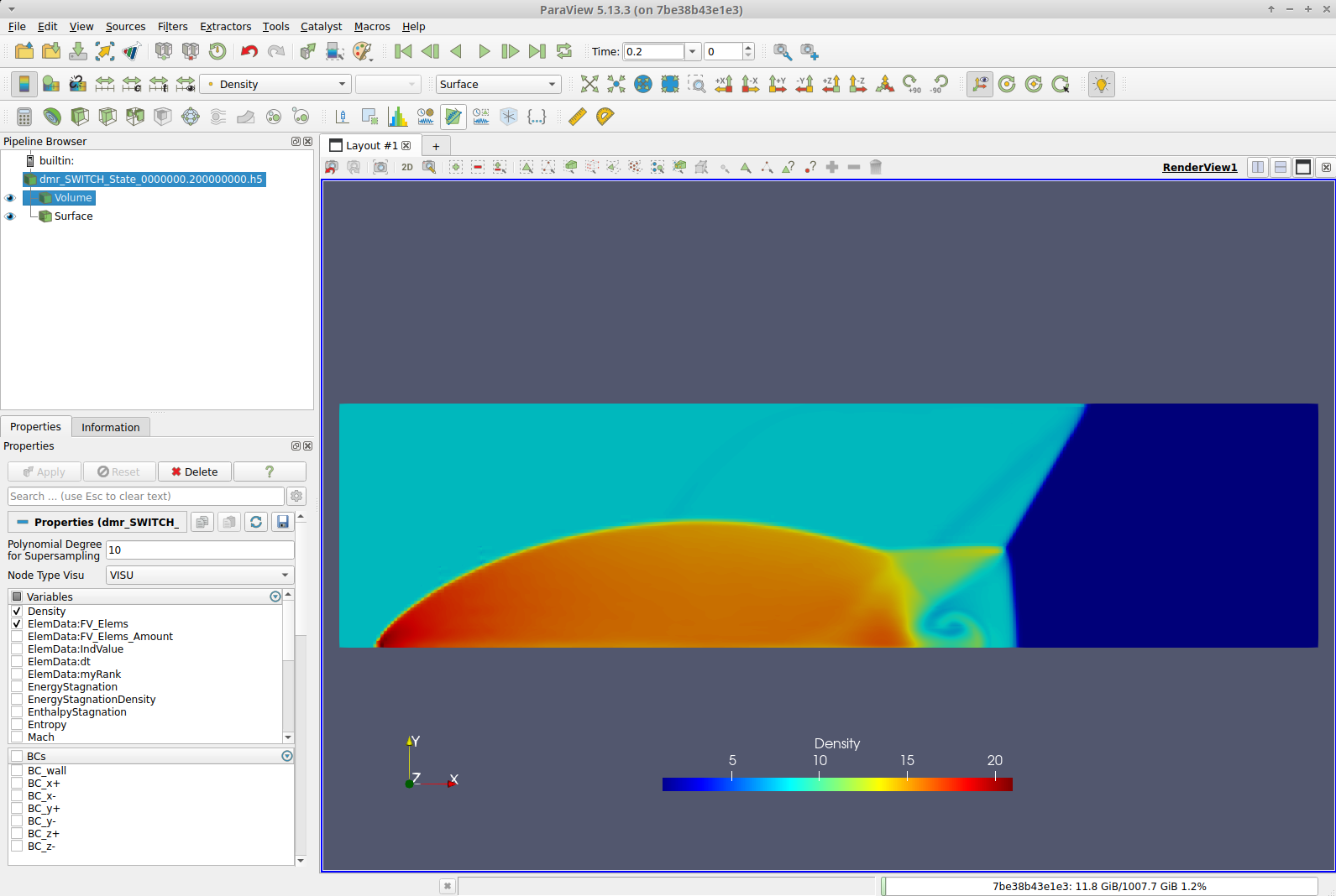
ParaView plugin to visualize the custom HDF5 state files of FLEXI directly (see Properties tab). — Fig. 6.1 ParaView plugin to visualize the custom HDF5 state files of **FLEXI** directly (see *Properties* tab).

Tip

Compiling ParaView from source may take 1-2 hours, depending on the system, and is prone to unmet dependencies errors. The Docker image in the GitHub container registry provides a complete FLEXI environment with HOPR / PyHOPE, ParaView and all dependencies pre-installed. The corresponding Dockerfile in .docker/ubuntu_24/ may serve as reference for a local FLEXI installation.

6.1.2. Mesh Swapping

The POSTI_SWAPMESH tool interpolates the solution of a StateFile or a TimeAverage file from one mesh to another, or from one polynomial degree to another. To do so, the parametric coordinates of the interpolation points of the new state are searched in the old mesh. For non-equal elements, a Newton algorithm is used to find the parametric coordinates of the interpolation points. Based on the found parametric coordinates, a high-order interpolation to the interpolation points in the new mesh is performed. Non-conforming meshes are allowed. A reference state can be given for areas in the target mesh which are not covered by the original mesh. The project name and therefore the file name is based on the original project name with _newMesh appended, the original file is therefore not overwritten.

For serial execution, the POSTI_SWAPMESH tool is invoked by entering

posti_swapmesh parameter_postiSwapmesh.ini <statefiles>

The tool also runs in parallel using OpenMP. To run in parallel, the environment variable OMP_NUM_THREADS=XXX needs to be set with the number of threads to be used, provided the compiler option LIBS_USE_OPENMP is enabled. In this case, the parallel execution is the same as the single execution.

A list of parameters used by the POSTI_SWAPMESH tool is listed in the table below. An example of the POSTI_SWAPMESH tool can be found in

./flexi/ini/swapmesh

Table 6.2 POSTI_SWAPMESH parameters.
Parameter	Possible Values	Description
MeshFileOld	none / MeshFileName.h5	Old mesh file (if different than the one found in the state file)
MeshFileNew	MeshFileName.h5	New mesh file
useCurvedsOld	T/F	Controls usage of high-order information in old mesh. Turn off to discard
useCurvedsNew	T/F	Controls usage of high-order information in new mesh. Turn off to discard
NInter	1 / 2 / 3 / …	Polynomial degree used for interpolation on new mesh (should be equal or higher than NNew) - the state will be interpolated to this degree and then projected down to NNew
NNew	1 / 2 / 3 / …	Polynomial degree used in new state files
NSuper	1 / 2 / 3 / …	Polynomial degree used for supersampling on the old mesh, used to get an initial guess for Newton’s method - should be higher than NGeo of old mesh
maxTolerance	value $\ge 0$	Tolerance used to mark points as invalid if outside of reference element more than maxTolerance
printTroublemakers	T/F	Turn output of not-found points on or off
RefState	complete conservative state vector	If a RefState is defined, this state will be used at points that are marked as invalid - without a RefState, the program will abort in this case
abortTolerance	value $\ge 0$	Tolerance used to decide if the program should abort if no RefState is given
ExtrudeTo3D	T/F	Perform an extrusion of a one-layer mesh to the 3D version Layer which is used in extrusion
ExtrudePeriodic	T/F	Perform a periodic extrusion of a 3D mesh to a mesh with extended z length

6.1.3. Recordpoints

For investigations with a high temporal resolution, such as frequency analyses, it is generally not practical to write complete state files with a high output frequency. Among other things, this would generate a considerable memory requirement and unnecessarily slow down the simulation due to frequent I/O operations. Numerical probes, here called record points, can therefore be used within FLEXI for high-frequency outputs in time. These represent point samples and can sample the flow variables with high temporal resolution at defined points in the domain. Multiple record points can be combined to form geometric shapes such as lines or surfaces.

The POSTI tools available for this are:

POSTI_RP_PREPARE: Definition of the points in the flow domain
POSTI_RP_VISUALIZE: Visualization of the variables recorded at runtime
POSTI_RP_EVALUATE: Subsequent evaluation of record points on existing volume solutions

To use the POSTI tools, the compile flag POSTI and the compile flag associated with the respective tool must be activated.

6.1.3.1. POSTI_RP_PREPARE

The POSTI_RP_PREPARE tool uses its own parameter file. This specifies the grouping of the recordpoints (individual points, lines, planes, …) and the associated mesh file for which the recordpoints will be defined. The parameters that can be used are documented in the table listed below. The available parameters can also be listed by using the help function

posti_preparerecordpoints --help

The tool can be executed as follows:

posti_preparerecordpoints parameter_recordpoints.ini

After successful execution, an additional h5 file is written with the name of the specified project name with postfix _RPSet. In order to record the data during the simulation, this file must be specified in the parameter file when executing FLEXI. If the doVisuRP option is used, the defined recordpoints are also written to a vtm file that can be viewed with Paraview.

To collect the date at the recordpoints locations during the simulation, the recordpoints functionality needs to be activated in the ini file of the FLEXI. This is done by setting RP_inUse = T.

The following exemplary options can be added to an existing parameter file:

RP_inUse            = T
RP_DefFile          = *_RPSet.h5
RP_SamplingOffset   = 10
RP_MaxMemory        = 100

Here, the specified RP_DefFile contains the element-local parametric recordpoint coordinates. This is the file generated by posti_preparerecordpoints. The option RP_SamplingOffset defines the multiple of timestep at which recordpoints are evaluated. Additionally, the RP_MaxMemory can be set. It defines the maximum memory in MiB to be used for storing recordpoint state history. If the memory is exceeded before regular I/O level, states are written to the file.

Table 6.3 POSTI_RP_PREPARE parameters.
Parameter	Possible Values	Description
ProjectName		Name used to identify the recordpoint file
MeshFile	MeshFileName.h5	Name of the mesh file
NSuper	1 / 2 / 3 / …	Number of Newton start values per element per direction.
maxTolerance	value $\ge 0$	Tolerance in parameter space at the element boundaries, required to mark a recordpoint as found.
doVisuRP	T/F	Write output file to visualize recordpoints.
GroupName		Name of the RP group (one for each group!)
Line_GroupID		ID of a straight line group, defined by start and end coordinates and the number of points along that line, used to allocate the definition to a specific group
Line_nRP		Number of RPs on line
Line_xstart		Coordinates of start of line
Line_xEnd		Coordinates of end of line
Circle_GroupID		ID of a circular group, used to allocate the definition to a specific group
Circle_nRP		Number of RPs along circle
Circle_Center		Coordinates of circle center
Circle_Axis		Axis vector of circle
Circle_Dir		Vector defining the start point on the circle
Circle_Radius		Radius of the circle
Circle_Angle		Angle from the start point, 360° is a full circle
CustomLine_GroupID		ID of a custom line, defined by an arbitrary number of RPs, used to allocate the definition to a specific group
CustomLine_nRP		Number of points on the custom line
CustomLine_x		Coordinates of the points on the custom line
Point_GroupID		ID of a point group, used to allocate the definition to a specific group
Point_x		Coordinates of the single point
Plane_GroupID		ID of a plane group, defined by the corner points and the number of points in both directions, used to allocate the definition to a specific group
Plane_nRP		Number of points in the plane
Plane_CornerX		Coordinates of the 4 corner points (x1,y1,z1,x2,y2,z2,…)
Box_GroupID		ID of a box group, defined by the corner points and the number of points in both directions, used to allocate the definition to a specific group
Box_nRP		Number of points in the box
Box_CornerX		Coordinates of the 8 corner points (x1,y1,z1,x2,y2,z2,…)
Sphere_GroupID		ID of a spherical group, with points on the circumference, used to allocate the definition to a specific group
Sphere_nRP		Number of points on the spere in phi and theta direction
Sphere_Center		Coordinates of sphere center
Sphere_Axis		Axis vector of sphere
Sphere_Dir		Vector defining the start point on the sphere
Sphere_Radius		Radius of the sphere
Sphere_Angle		Phi angle of the sphere (360° is a full sphere)
BLPlane_GroupID		ID of a boundary layer group - works like a plane group, but the plane is created by projecting the points of a spline to the nearest boundary and extruding the plane along the normal with a stretching factor, used to allocate the definition to a specific group
BLPlane_nRP		Number of RPs along and normal to the boundary
BLPlane_nCP		Number of control points defining the spline (at least two)
BLPlane_CP		Coordinates of the spline control points
BLPlane_fac		Factor of geometrical stretching in wall-normal direction
BLPlane_height		Wall-normal extend of the plane for each control point
BLBox_GroupID		ID of a boundary layer group - works like a box group, but the box is created by projecting the points of a spline to the nearest boundary and extruding the box along the normal with a stretching factor, used to allocate the definition to a specific group
BLBox_nRP		Number of RPs along and normal to the boundary
BLBox_nCP		Number of control points defining the spline (at least two). Defined once per BLBox
BLBox_nSP		Number of shifted splines (at least one), linear interpolation between the splines in shifted direction (linear extrusion)
BLBox_CP		Coordinates of the spline control points. nCPxnSP needed.
BLBox_fac		Factor of geometrical stretching in wall-normal direction.
BLBox_height		Wall-normal extend of the box for each control point

Exemplary applications of POSTI_RP_PREPARE can be found in the following tutorials: Flow Around a Cylinder, Flow Around a NACA0012 Airfoil Sample parameter files can also be found here.

6.1.3.2. POSTI_RP_VISUALIZE

During the runtime of the simulation, ProjectName_RP_*.h5 files are written. These files contain the raw data collected during the simulation. Using the posti_visualizerecordpoints tool, the raw data can be further post-processed. The tool takes one or more of the recordpoint files and combines them into a single time series. From the conservative variables that are stored during the simulation, all available derived quantities can be computed. Additionally, several more advanced post-processing algorithms are available. This includes calculation of time averages, FFT, and PSD values and specific boundary layer properties.

The posti_visualizerecordpoints tool is designed for single execution only and can be executed as follows:

posti_visualizerecordpoints parameter_visuRP.ini projectname_RP_*.h5

The parameters that can be used are documented in the table listed below. The available parameters can also be listed by using the help function

posti_visualizerecordpoints --help

Table 6.4 POSTI_RP_VISUALIZE parameters.
Parameter	Possible Values	Description
ProjectName		Name of the project
GroupName		Name(s) of the group(s) to visualize, must be equal to the name given in preparerecordpoints tool
VarName		Variable name to visualize
RP_DefFile		Path to the *RPset.h5 file
usePrims	T / F	Set to indicate that the RP file contains the primitive and not the conservative variables
meshScale		Specify a scalar scaling factor for the RP coordinates
OutputTimeData	T / F	Should the time series be written? Not compatible with TimeAvg and FFT options!
OutputTimeAverage	T/ F	Should the time average be computed and written?
doFluctuations	T / F	Should the fluctuations be computed and written?
equiTimeSpacing	T / F	Set to interpolate the temporal data to equdistant time steps (always done for operations requiring FFTs)
OutputPoints	T / F	General option to turn off the output of points
OutputLines	T / F	General option to turn off the output of lines
OutputPlanes	T / F	General option to turn off the output of planes
OutputBoxes	T / F	General option to turn off the output of boxes
doFFT	T / F	Calculate a fast Fourier transform of the time signal
doPSD	T / F	Calculate the power spectral density of the time signal
nBlocks		Specify the number of blocks over the time signal used for spectral averaging when calculating spectral quantities
SamplingFreq		Instead of specifying the number of blocks, the sampling frequency in combination with the block size can be set - the number of blocks will then be calculated.
BlockSize		Size of the blocks (in samples) if sampling frequency is given
CutoffFreq		Specify smallest considered frequency in spectral analysis
hanning	T / F	Set to use the Hann window when performing spectral analysis
doTurb	T / F	Set to compute a temporal FFT for each RP and compute turbulent quantities like the kinetic energy over wave number
Box_doBLProps	T / F	Set to calculate seperate boundary layer quantities for boundary layer planes
Box_BLvelScaling		Choose scaling for boundary layer quantities. 0: no scaling, 1: laminar scaling, 3: turbulent scaling
Plane_doBLProps	T / F	Set to calculate seperate boundary layer quantities for boundary layer planes
Plane_BLvelScaling		Choose scaling for boundary layer quantities. 0: no scaling, 1: laminar scaling, 3: turbulent scaling
RPRefState		Refstate required for computation of e.g. cp.
RefState		State(s) in primitive variables (density, velx, vely, velz, pressure).
Box_LocalCoords	T / F	Set to use local instead of global coordinates along boxes
Box_LocalVel	T / F	Set to use local instead of global velocities along boxes
Plane_LocalCoords	T / F	Set to use local instead of global coordinates along planes
Plane_LocalVel	T / F	Set to use local instead of global velocities along planes
Line_LocalCoords	T / F	Set to use local instead of global coordinates along lines
Line_LocalVel	T / F	Set to use local instead of global velocities along lines
Line_LocalVel_vec		Vector used for local velocity computation along line
doFilter	T / F	Set to perform temporal filtering for each RP
FilterWidth		Width of the temporal filter
FilterMode		Set to 0 for low pass filter and to 1 for high pass filter
TimeAvgFile		Optional file that contains the temporal averages that should be used
SkipSample		Used to skip every n-th RP evaluation
OutputFormat		Choose the main format for output. 0: ParaView, 2: HDF5
doEnsemble	T / F	Set to perform ensemble averaging for each RP
EnsemblePeriod		Periodic time to be used for ensemble averaging
UseNonDimensionalEqn	T / F	Set true to compute R and mu from bulk Mach Reynolds (nondimensional form.
kappa	1.4	Heat capacity ratio / isentropic exponent
R	287.058	Specific gas constant
Pr	0.72	Prandtl number
mu0	0.0	Dynamic Viscosity
Ts	110.4	Sutherland’s law for variable viscosity: Ts
Tref	273.15	Sutherland’s law for variable viscosity: Tref
ExpoSuth	1.5	Sutherland’s law for variable viscosity: Exponent

Exemplary applications of POSTI_RP_PREPARE can be found in the following tutorials: Flow Around a Cylinder, Flow Around a NACA0012 Airfoil Sample parameter files can also be found here.

6.1.3.3. POSTI_RP_EVALUATE

The POSTI_RP_EVALUATE tool can be used to extract data for a given simulation at the defined positions for a given RP_DefFile. For this purpose, the recordpoints can be defined as described in section POSTI_RP_PREPARE and the data can be extracted. It is possible to extract data not only form StateFiles but also e.g. from TimeAverageFiles. By default, the data set DG_Solution is read, which can be used to extract data from StateFiles. To extract data from TimeAverageFiles, a corresponding data set like Mean or Fluc needs to be specified in the parameter file option RecordpointsDataSetName. Using the following command the data can be extracted at the recordpoint positions:

posti_evaluaterecordpoints [parameter.ini] <solutionfiles>

The tool also runs in parallel by prepending mpirun -np <no. processors> to the above command, as usual, provided the compiler option LIBS_USE_MPI is enabled.

mpirun -np <no. processors> posti_evaluaterecordpoints [parameter.ini] <solutionfiles>

After the execution of the posti_evaluaterecordpoints tool, a ProjectName_RP_*.h5 file is written. This file is similar to the recordpoint files written during runtime. Therefore, these files can be visualized as described in section POSTI_RP_VISUALIZE.

Important

The MPI-parallel HDF5 implementation internally uses a signed 32-bit integer, restricting the maximum chunk size to $2\, GB$ per thread. When post-processing with activated LIBS_USE_MPI flag, especially with large cases and large files as is often the case with TimeAverage files, the file size of approximately $2\, GB$ per core must not be exceeded. In this case, the number of cores used must be increased for MPI-parallel executable POSTI tools, or POSTI must be compiled with LIBS_USE_MPI=OFF.

The parameters for this POSTI tool are listed in the table below.

Table 6.5 POSTI_RP_EVALUATE parameters.
Parameter	Possible Values	Description
RP_inUse	T / F	Set true to compute solution history at points defined in recordpoints file
RP_DefFile	ProjectName_RPSet.h5	File containing element-local parametric recordpoint coordinates and structure
RP_MaxMemory	100	Maximum memory in MiB to be used for storing recordpoint state history. If memory is exceeded before regular IO level states are written to file
RP_SamplingOffset	1	Multiple of timestep at which recordpoints are evaluated
RecordpointsDataSetName	DG_Solution / Mean / Fluc / …	If no state files are given to evaluate, specify the data set name to be used here

The available parameters can also be listed by using the help function

posti_evaluaterecordpoints --help

6.1.4. Time Averaging

The following tools allow to handle either time-averaged high-frequency data averaged during the simulation or averages the states files written by FLEXI over time.

6.1.4.1. POSTI_MERGETIMEAVERAGES

The POSTI_MERGETIMEAVERAGES tool averages several FLEXI State or TimeAverage files. If TimeAverage files are the input, each file is weighted with its time averaging period. State files are all weighted equally. All HDF5 data sets are averaged and no additional parameter file is required.

The basic usage of this tool is as follows, with the three optional flags detailed in the table below.

posti_mergetimeaverages --start=[starttime] --end=[endtime] --coarsen=[factor] [inputfile1.h5 inputfile2.h5 ...]

Table 6.6 Optional flags of POSTI_MERGETIMEAVERAGES.
Flag	Default Value	Description
start	$-\infty$	Start time for time averaging. Input files with a timestamp prior to the start time are skipped.
end	$+\infty$	End time for time averaging. Input files with a timestamp after the end time are skipped.
coarsen		Number of successive input files to consider for one time average. Default is to consider all input files.

6.1.4.2. POSTI_CALCFLUCTUATIONS

The POSTI_CALCFLUCTUATIONS tool calculates fluctuations from the Mean and MeanSquare given in the (merged) TimeAverage files. Fluctuations are then written into an additional data set in the same HDF5 file. All applicable fluctuations are calculated and no additional parameter file is required. This results in the following basic usage of the tool:

posti_calcfluctuations [timeavgfile1.h5 timeavgfile2.h5 ...]

In general, the total value of a variable $U$ can be split into the temporal mean $u$ and the fluctuating part $u'$, that is $U = u+u'$ with $u=<U>$ and $<u'>=0$. During a simulation with CalcTimeAverage=T, FLEXI will write two data sets: the mean of a variable, $<U>$, and the mean of the squared variable, $<UU>$. To compute the fluctuations, i.e. the mean of the squared fluctuations $<u'u'>$, based on these two quantities, we make use of the following relation:

(6.1)\[\begin{gather} <UU> = <(u+u')(u+u')> = <uu> + <2uu'> + <u'u'> = uu + <u'u'> \\ \Rightarrow \quad <u'u'> = <UU> - uu \end{gather}\]

6.1.4.3. POSTI_CHANNEL_FFT

The POSTI_CHANNEL_FFT tool calculates the mean velocity and Reynolds stress profiles of the turbulent channel flow test case by averaging both in the direction parallel to the wall and by averaging the upper and lower half of the channel. Furthermore, kinetic energy spectra dependent on the distance to the wall are computed.

The tool relies on a separate parameter file and comes with the basic usage

posti_channel_fft [parameter_channelfft.ini] [statefile1.h5 statefile2.h5 ...]

The available parameters can be displayed by passing the --help flag and are listed in the table below.

Table 6.7 POSTI_CHANNEL_FFT parameters.
Parameter	Possible Values	Description
N		Polynomial degree of computation to represent to solution.
GroupSize	0 / 2 / 4 / … (no. procs per node)	Defines the size of MPI subgroups, used to e.g. perform grouped IO, where group master collects and outputs data.
gatheredWrite	T / F	Set true to activate gathered HDF5 IO for parallel computations. Only local group masters will write data after gathering from local slaves.
MeshFile	MeshFileName.h5	(relative) path to meshfile (mandatory).
useCurveds	T / F	Controls usage of high-order information in mesh. Turn off to discard high-order data and treat curved meshes as linear meshes.
interpolateFromTree	T / F	For non-conforming meshes, built by refinement from a tree structure, the metrics can be built from the tree geometry if it is contained in the mesh. Can improve free-stream preservation.
meshScale		Scale the mesh by this factor (shrink for <1.0 / enlarge for >1.0).
meshdeform	T / F	Apply simple sine-shaped deformation on cartesion mesh (for testing).
crossProductMetrics	T / F	Compute mesh metrics using cross product form. Caution: in this case free-stream preservation is only guaranteed for N=3*NGeo.
debugmesh	0 / 3	Output file with visualization and debug information for the mesh: 0 = no visualization, 3 = Paraview binary
BoundaryName		Names of boundary conditions to be set (must be present in the mesh!). For each BoundaryName a BoundaryType needs to be specified.
BoundaryType	(BC_TYPE,BC_STATE)	Type of boundary conditions to be set.
writePartitionInfo	T / F	Write information about MPI partitions into a file.
NGeoOverride	-1 / 1 / 2 / …	Override switch for NGeo. Interpolate mesh to different NGeo: <1 = off, >0 = interpolate
OutputFormat	0 / 2	Choose the main format for output: 0 = Tecplot, 2 = HDF5
NCalc		Polynomial degree to perform DFFT on.
Re_tau		Reynolds number based on friction velocity and channel half height.

An exemplary application of the POSTI_CHANNEL_FFT tool, along with a sample parameter file, can be found in the tutorial Plane Turbulent Channel Flow.

6.2. Tools Folder

The scripts provided in the tools folder are generally not part of the tutorials. They are briefly described below, where the path to the files (of the form $FLEXIROOT/tools/SUBDIR/) is omitted. For most Python tools, possible arguments and syntax can be shown with the -h argument:

python3 [toolname.py] -h

6.2.1. Animate Tool

The Python script animate_paraview.py creates movies from a series of state files using pvbatch, a GUI-less interface to ParaView. It requires ParaView to be installed on the system and the directory containing the pvbatch executable to be a part of the $PATH variable.

Before running this script, you need to visualize one of the considered FLEXI state files in ParaView and save the current view via Save State..., e.g. under the name pvstate.pvsm. The basic command to run the script is

python3 animate_paraview.py -l [pvstate.pvsm] -r [path_to_posti_paraview_plugin] [statefile1.h5 statefile2.h5 ...]

This will output a .png-file for each HDF5 file given as input and concatenate them into a video. The video generation relies on the MEncoder tool and can be turned off via the -n flag. In order to visualize a set of .vtu-files, e.g., from the posti_visu output, omit the -r argument and pass .vtu-files instead of .h5-files. Further options can shown with the -h argument.

There are further tools for image handling in this folder, which all can be called with the -h flag to show the complete list of possible arguments:

concatenatepics.py stitches several pairs of images, e.g. to create a time series of stitched images from two time series of images

python3 concatenatepics.py -d e -p left*.png  -a right*.png

crop.py crops several images to the same size, simply pass all images as arguments:

python3 crop.py [image*.png]

pics2movie.py creates a movie from several images using the mencoder tool (which is also done as part of the animate_paraview.py script)

python3 pics2movie.py [image*.png]

6.2.2. Convergence Tests

The Python scripts convergence.py and convergence_grid.py provide automated convergence tests for $p$- and $h$-convergence, respectively. They call FLEXI repeatedly on a given parameter file while modifying the polynomial degree $N$ or the mesh file, and compute the Experimental Order of Convergence (EOC) automatically. The basic command for $p$-convergence is

convergence [path/to/flexi] [parameter.ini]

where convergence can be replaced by convergence_grid for $h$-convergence. Further options can again be shown with the -h option.

Note that for $h$-convergence, the mesh names are hard-coded to the form CART_HEX_PERIODIC_MORTAR_XXX_2D_mesh.h5, where XXX denotes the number of elements in each direction, and MORTAR and 2D are optional.

6.2.3. Userblock Tool

The userblock contains complete information about a FLEXI run (git branch of the repository, differences to that branch, cmake configuration and parameter file) and is prepended to every .h5 state file. The parameter file is prepended in ASCII format, the rest is binary and is generated automatically during the build process with the generate_userblock.sh script. It can be extracted and printed using the extract_userblock.py script. Its basic usage is

python3 extract_userblock.py -XXX [statefile.h5]

where -XXX can be replaced by

-s to show all available parts of the userblock (such as CMAKE or GIT BRANCH)
-a to print the complete userblock
-p [part] to print one of the parts listed with the -s command.

The second python tool in this folder is rebuild.py. It extracts the userblock from a state file and builds a FLEXI repository and binary identical to the one that state file was created with. In order to do so, it clones a FLEXI git repository, checks out the given branch, applies the stored changes to the git HEAD and builds FLEXI with the stored cmake options. If run with the parameter file given in the INIFILE part of the userblock, this binary should reproduce the same results/behavior (possible remaining sources of different output are, for example, differences in restart files, compilers, linked libraries or machines). The basic usage is

python3 rebuild.py [dir] [statefile.h5]

where dir is an empty directory that the repository is cloned into and where the flexi executable is built, and statefile.h5 is the state file whose userblock is used to rebuild the flexi executable. Help can be shown via -h for both userblock scripts.