5.6. SOD Shock Tube
The Sod shock tube example [22] is one of the most basic test cases to investigate the shock capturing capabilities of a CFD code. An initial discontinuity is located in the middle of the one dimensional domain \(x \in [0,1]\). The left and right states are given by \(\rho=1, v=0, p=1\) and \(\rho=0.125, v=0, p=0.1\). The tutorial is located at tutorials/sod. These states are already set as RefState in the parameter_flexi.ini file.
5.6.1. Mesh Generation
In the tutorial directory, we provide the necessary mesh files, along with a parameter files for HOPR to generate these meshes. You can recreate any mesh by running the following command. A full tutorial on how to run HOPR is available at the [HOPR documentation][hopr].
hopr parameter_hopr.ini
5.6.2. Build Configuration
This example requires the Finite Volume (FV) shock capturing and the Euler equations. In this tutorial, we will investigate the shock capturing based on switching the DG representation to FV sub-cells.
Therefore, [FLEXI][flexi] should be compiled either with the sod preset using the following command
cmake -B build --preset sod
cmake --build build
5.6.3. Simulation Parameters
The parameter file to run the simulation is supplied as parameter_flexi.ini.
5.6.3.1. Finite Volume Shock Capturing
The options for the Finite Volume shock capturing are contained in the ‘FV-Subcell’ section.
! ============================================================ !
! FV-Subcell
! ============================================================ !
IndicatorType        = Persson
IndVar               = 1       ! first conservative (density)
                               ! used for indicator evaluation
IndStartTime         = 0.001   ! until this time FV is used in
                               ! the whole domain

FV_LimiterType       = MinMod
FV_IndUpperThreshold = -3.     ! upper threshold (if IndValue
                               ! above this value, switch to FV)
FV_IndLowerThreshold = -4.     ! lower threshold (if IndValue
                               ! below this value, switch to DG)
The IndicatorType parameter sets the type of indicator function used to detect DG elements containing discontinuities. For this case, the Persson indicator [23] is applied, an element-local indicator that compares the different modes of the DG polynomial. If the relative content in the highest mode is high compared to the amount in the lower modes, the DG polynomial may show oscillatory behavior. All indicator functions return a high value for “troubled” with discontinuities and low values for smooth elements. The variable IndVar specifies the index within the conservative variable vector used to evaluate the indicator function. Typically, pressure (index 6) is a good choice; however, for this test case, density is used instead. IndStartTime specifies a time during which the actual indicator function is overwritten by a high value to force the use of FV elements everywhere. This helps capture initial discontinuities placed exactly at element boundaries, as element-local indicators like Persson can not detect these discontinuities. FV_LimiterType sets the limiter used in the second-order FV reconstruction. FV_IndUpperThreshold and FV_IndLowerThreshold define thresholds for deciding in which elements are represented by the DG method and where the FV sub-cell scheme should be used. While a single threshold can theoretically suffice, it often leads to continuous switching between the DG and the FV schemes. To avoid this, switching to FV only occurs if the indicator exceeds the upper threshold. Switching back to DG only happens if the indicator value falls below the lower threshold.
5.6.4. Simulation and Results
We proceed by running the code with the following command.
flexi parameter_flexi.ini
This test case generates \(5\) state files name sod_State_>TIMESTAMP>.h5 for \(t=0.0, 0.05, 0.10, 0.15, 0.20\).
5.6.4.1. Visualization
FLEXI relies on ParaView for visualization. In order to visualize the FLEXI solution, its format has to be converted from the HDF5 format into another format suitable for Paraview. FLEXI provides a post-processing tool posti_visu which generates files in VTK format with the following command.
posti_visu parameter_postiVisu.ini parameter_flexi.ini sod_State_0*
posti_visu generates two types of files which can be loaded into ParaView. vtu files contain either DG or the FV part of the solution. The vtm-files combine the DG and FV vtu-file of every timestamp. It is thus recommended to load the vtm-files into ParaView.
For this one-dimensional test case, apply the Plot Over Line filter in ParaView. When setting up the filter, choose the X Axis as the line direction to create a line plot of the variable values along this axis. The resulting plot should resemble the one shown in Fig. 5.21.
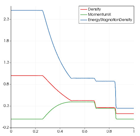
Fig. 5.21 Solution of the Sod shock tube at \(t=0.2\).