5.7. Double Mach Reflection
The Double Mach Reflection is a classical test case to investigate the abilities of a numerical scheme to represent shocks and contact discontinuities. It was proposed by Colella and Woodward [24] and considers a Mach 10 oblique shock wave that hits a reflecting wall. The initial conditions are given by the Rankine-Hugoniot conditions
where the wall at the bottom starts at \(x_0= \frac{1}{6}\) and the computational domain \(\Omega = [0,4] \times [0,1]\) is discretized by an equidistant Cartesian mesh. This tutorial is located in the folder tutorials/dmr.
5.7.1. Mesh Generation
In the tutorial directory, we provide the necessary mesh files, along with a parameter files for HOPR to generate these meshes. You can recreate any mesh by running the following command. A full tutorial on how to run HOPR is available at the [HOPR documentation][hopr].
hopr parameter_hopr.ini
5.7.2. Flow Simulation
This example requires the finite volume (FV) shock capturing. Two variants of the shock capturing are implemented in FLEXI, which are both based on the FV sub-cell approach. This approach subdivides each DG element into FV sub-cells, where each cell corresponds to one degree of freedom of the initial DG element. Thus, the total number of degrees of freedom is constant throughout the simulation, while the DG and the FV operator are chosen independently for each individual element.
The first variant of the FV sub-cell approach switches DG elements into the FV sub-cell representation such that the element-local solution is either a smooth polynomial (DG representation) or piecewise constant (FV sub-cell), as detailed in [3]. The second variant of the FV sub-cell approach blends the DG operator with the FV operator, while the solution itself always remains a DG polynomial, see [4] for more details. In the following, both approaches will be applied to simulate the Double Mach Reflection.
5.7.2.1. Finite Volume Switching
In the switching-based shock capturing, the element-local solution is either given in DG representation (FV_Elems=0) or interpolated to piecewise constant FV sub-cells (FV_Elems=1).
5.7.2.1.1. Build Configuration
The FV switching is enabled through the build option FLEXI_FV=SWITCH, the corresponding CMake preset cmd_fvswitch is applied by running
cmake -B build --preset dmr_fvswitch
cmake --build build
5.7.2.1.2. Simulation Parameters
The simulation setup is defined in parameter_flexi_switch.ini and includes parameters for the shock capturing via switching.
! ============================================================ !
! FV-Subcell
! ============================================================ !
IndicatorType        = Jameson
IndVar               = 6       ! sixth variable (pressure)
                               ! used for indicator evaluation
FV_LimiterType       = 1       ! MinMod
FV_IndUpperThreshold = 0.010   ! upper threshold (if IndValue
                               ! above this value, switch to FV)
FV_IndLowerThreshold = 0.005   ! lower threshold (if IndValue
                               ! below this value, switch to DG)
FV_toDG_indicator    = T
FV_toDG_limit        = -5.5
FV_IniSupersample    = T
The IndicatorType parameter sets the type of indicator function used to detect DG elements containing discontinuities. For this case, the Jameson indicator [23] is applied, an adaptation of the switching function of the Jameson-Schmidt-Turkel scheme [25] to FV sub-cells. In contrast to the Persson indicator, it is not element-local and therefore more robust for traveling discontinuities. All indicator functions return a high value for “troubled” with discontinuities and low values for smooth elements. The variable IndVar specifies the index within the variable vector used to evaluate the indicator function. Typically, pressure (index 6) is a good choice and also used here. FV_toDG_indicator enables an additional Persson indicator [23] for the switch from FV to DG. When an FV element is marked for transition to DG, it is temporarily converted to a DG element and the Persson indicator is evaluated for this DG polynomial to test if the polynomial is oscillating. Only in the case of a non-oscillatory solution, the solution is converted to DG. Otherwise, the element retains the FV representation. This improves the simulation stability when indicator functions defined on the FV sub-cells are used. In the given case, the Jameson indicator only considers oscillations between adjacent degrees of freedom (DOFs), which may miss certain high-frequency oscillations in the polynomial. The FV_toDG_limit parameter is then used as threshold for additional Persson indicator, restricting the FV to DG transition to indicator values below this choice. During initialization, by default the solution is initialized as DG polynomials for all elements. In a second, step, the indicator function is evaluated to identify troubled elements which are then converted to an FV representation. This can cause issues if discontinuities lie inside DG elements which leads to strongly oscillating polynomials and invalid solutions, e.g., negative density, even after converting these oscillating polynomials to FV. The FV_IniSupersample option enables a super-sampling of the initial solution for every FV sub-cell, which removes the mentioned problems with oscillating polynomials. The mean value of every FV sub-cell is computed by evaluating the initial solution in \((N+1)\) equidistant points per dimension inside the sub-cell and then taking the arithmetic mean value.
5.7.2.2. Simulation and Results
We proceed by running the code with the following command.
flexi parameter_flexi_switch.ini
This test case generates \(11\) state files name dmr_SWITCH_State_<TIMESTAMP>.h5 for \(t=0.0, 0.02, \ldots, 0.20\).
5.7.2.3. Visualization
FLEXI relies on ParaView for visualization. In order to visualize the FLEXI solution, its format has to be converted from the HDF5 format into another format suitable for Paraview. FLEXI provides a post-processing tool posti_visu which generates files in VTK format with the following command.
posti_visu parameter_postiVisu.ini parameter_flexi_switch.ini dmr_SWITCH_State_0000000.*
posti_visu generates two types of files which can be loaded into ParaView. vtu files contain either DG or the FV part of the solution. The vtm-files combine the DG and FV vtu-file of every timestamp. It is thus recommended to load the vtm-files into ParaView. The result at \(t=0.2\) should look like in figure Fig. 5.22.
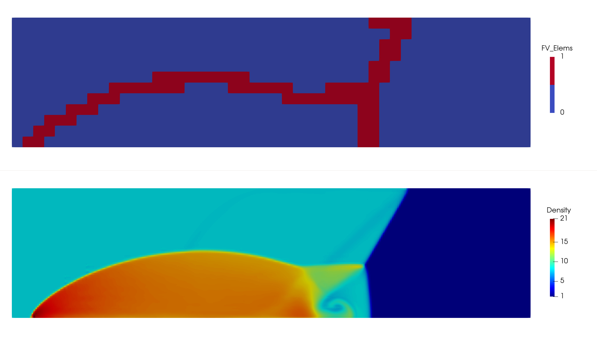
Fig. 5.22 Distribution of DG and FV elements (top) and density (bottom) of Double Mach Reflection at \(t=0.2\).
5.7.2.4. Finite Volume Blending
Next, we will investigate the blending approach. In this tutorial we use an entropy-stable split formulation to ensure the stability of the FV blending approach, with more details on the split formulation given later in section Plane Turbulent Channel Flow. For the FV sub-cell blending, the elements are not switched completely to the FV operator, but instead the DG operator \(R_{DG}\) and FV operator \(R_{FV}\) are blended as
with the blending coefficient \(\alpha\). Instead of switching between a DG and a FV discretization, the blending allows a continuous transition between the DG and FV operators. The blending factor is computed based on the indicator proposed by [4], which is parameter-free and does not require any parameters to be tuned by the user.
5.7.2.4.1. Build Configuration
The FV blending is enabled through the build option FLEXI_FV=BLEND. The FV blending requires selecting the Gauss-Lobatto node set by setting FLEXI_NODETYPE=GAUSS-LOBATTO and to enable the split-form DG with FLEXI_SPLIT_DG=ON. FLEXI should be compiled using the dmr_fvblend present.
cmake -B build --preset dmr_fvblend
cmake --build build
5.7.2.4.2. Simulation Parameters
The simulation setup is defined in parameter_flexi_blend.ini and the simulation parameters specific to the FV blending approach are summarized below.
! ============================================================ !
! FV-Subcell
! ============================================================ !
IndicatorType        = Jameson
IndVar               = 6       ! sixth variable (pressure)
                               ! used for indicator evaluation
FV_LimiterType       = 1       ! MinMod
FV_alpha_min         = 0.01    ! Lower bound for alpha (all
                               ! elements below threshold are
                               ! treated as pure DG)
FV_alpha_max         =  0.5    ! Maximum value for alpha. All
                               ! blending coefficients exceeding
                               !  this value are clipped
FV_alpha_ExtScale    =  0.5    ! Scaling factor by which the
                               ! blending factor is scaled when
                               ! propagated to its neighbor.
                               ! Has to be between 0 and 1.
FV_nExtendAlpha      =    1    ! Number of times this propagation
                               ! of the blending should be performed
                               ! (number of element layers).
                               ! Higher values correspond to a wider
                               ! sphere of influence.
FV_doExtendAlpha     =    T    ! Blending factor is prolongated
                               ! into neighboring elements
5.7.2.5. Simulation and Results
Similarly to the switching-based approach, we proceed by running the code with the following command.
flexi parameter_flexi_blend.ini
This test case generates \(11\) state files name dmr_BLEND_State_<TIMESTAMP>.h5 for \(t=0.0, 0.02, \ldots, 0.20\).
5.7.2.6. Visualization
FLEXI relies on ParaView for visualization. In order to visualize the FLEXI solution, its format has to be converted from the HDF5 format into another format suitable for Paraview. FLEXI provides a post-processing tool posti_visu which generates files in VTK format with the following command.
posti_visu parameter_postiVisu.ini parameter_flexi_blend.ini dmr_BLEND_State_0000000.*
As the solution is always represented by DG polynomials. posti_visu generated only the DG part of the solution. Thus, load the generated vtm-files into ParaView. The result at \(t=0.2\) should look like in figure Fig. 5.23.
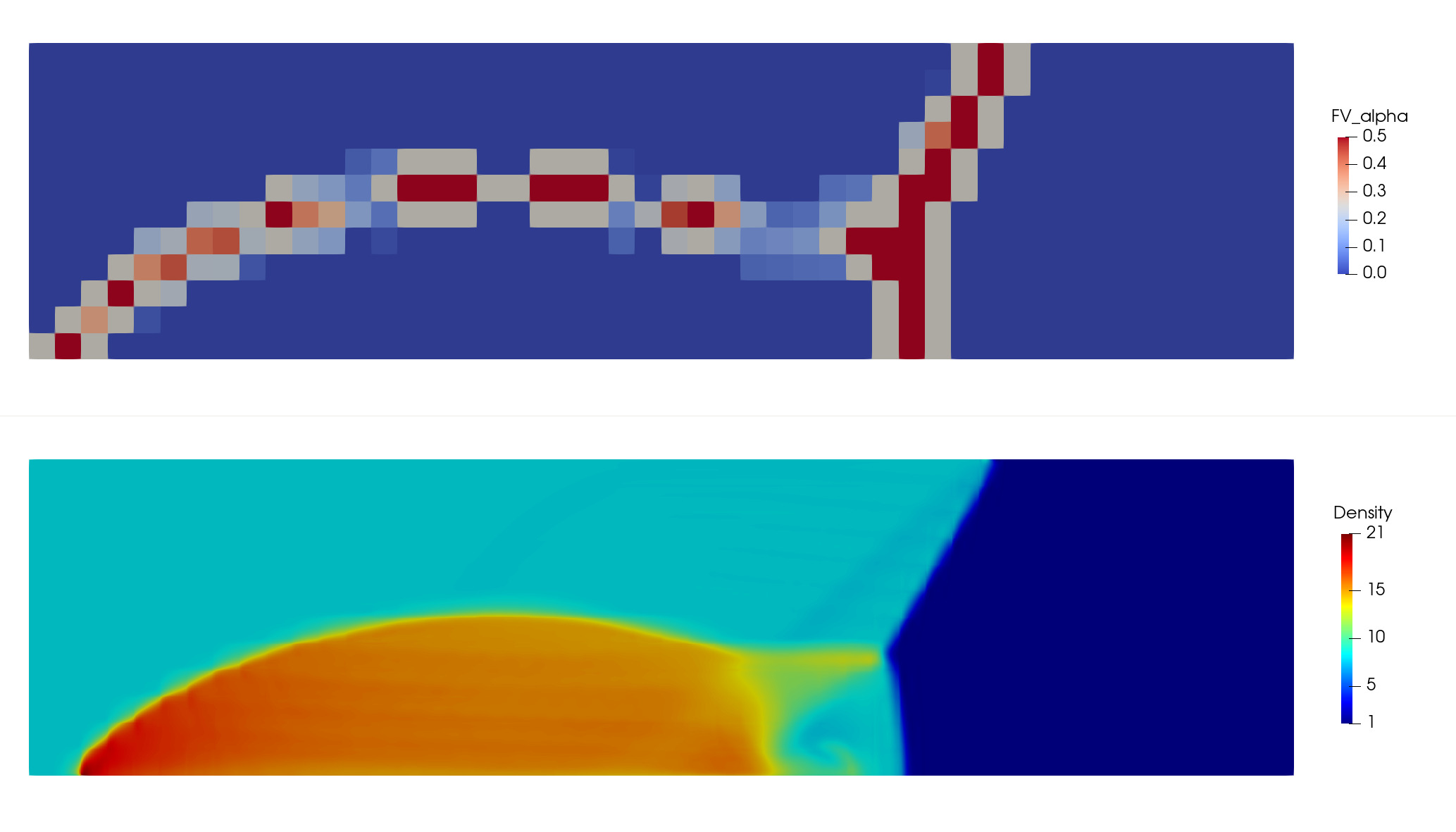
Fig. 5.23 Distribution of the blending factor \(\alpha\) between the DG and FV operators (top) and density (bottom) of Double Mach Reflection at \(t=0.2\).