5.3. Convergence Test

This tutorial demonstrates how to compute the order of convergence for FLEXI. The process is fully scripted, allowing for multiple runs across varied grids and polynomial degrees, with the convergence order calculated automatically. Once the runs are completed, the script generates a plot of the corresponding \(L_2\) error norms and saves it in the directory from which the convergence test was executed. This script is written in Python3.

5.3.1. Manufactured Solution

To compute the order of convergence in FLEXI, we apply a benchmark test where an exact analytical solution is known. For this tutorial, we use the method of manufactured solutions. A detailed description is found in Roache [18]. In this method, a smooth function is proposed the solution to the equation system. Since this function generally does not provide a solution to the system of equations, a source term is calculated to force the corresponding solution. The source term is derived analytically and inserted into the equation system, cf. for the continuity equation, we obtain

\[\rho_t + (\rho u)_x = Q(x,t) \quad \text{with} \quad \rho = A + \sin(B(x,t)) \quad \text{and} \quad u = \text{const}.\]

The source term must be added within the time integration loop of the flow solver. In FLEXI sine waves are advected in the density using a constant velocity field. The actual source terms to be considered depend on the equation system, that is whether Euler or Navier-Stokes equations are used.

5.3.2. Mesh Generation

In the tutorial directory, we provide the necessary mesh files, along with a parameter files for HOPR to generate these meshes. You can recreate any mesh by running the following command.

hopr parameter_hopr.ini

Non-Conforming Meshes

FLEXI supports non-conforming meshes with mortar interfaces. For the convergence test, parameter files for four mortar meshes are also provided, recognizable through filenames containing the term MORTAR. To use the convergence test script, simply open the script file at tools/convergence_test/convergence_grid and replace the mesh filenames. After that, the script can be executed in the same manner as for the conforming meshes.

5.3.3. Inviscid Convergence Test

We focus first on the convergence test without viscous terms, i.e. conference for the Euler equations.

5.3.3.1. Manufactured Solution

The manufactured solution for the Euler equation reads as

\[\rho = A (1 + B\sin(\Omega |\underline{x} - \underline{v}t|)) \quad \text{with} \quad A,B,\Omega,\underline{v} = const.\]

Since we are working with the Euler equations, the source term is zero, \(Q(x,t) \equiv 0\). To investigate the order of convergence for a given polynomial degree \(N\), the mesh resolution must be progressively refined. We provide meshes with \(1\), \(2\), \(4\), and \(8\) elements in each spatial direction together with the corresponding parameter files in the directory parameter_hopr. Fig. 5.4 displays an exemplary mesh used for the convergence test and the flow field solution of the density.

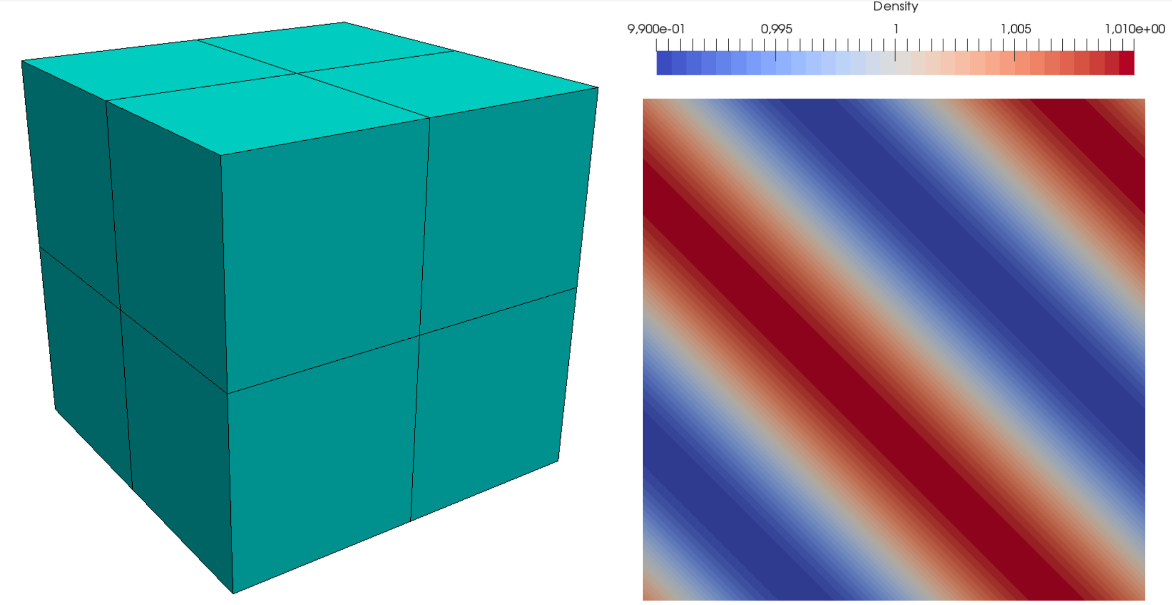
../../_images/convtest_result_mesh.jpg — Fig. 5.4 Convergence test: Mesh and flow field solution of the density.

5.3.3.2. Compiler Options

FLEXI should be compiled with the convtest_inviscid preset using the following commands.

cmake -B build --preset convtest_inviscid
cmake --build build

5.3.3.3. Simulation Parameters

The inviscid convergence test is run from the parameter file parameter_convtest_flexi.ini. Essentially, any valid parameter file can be used since a manufactured solution is simulated. This allows to test the various methods and features of the code and investigate their order of convergence. However, for this tutorial, we restrict the parameter file to a simple baseline test case. The default settings for the time integration are displayed in Table 5.4.

Table 5.4 Numerical settings used for the inviscid convtest.
Variable	Value	Description
N_Analyze	at least \(2N\)	Number of interpolation nodes for the analyze routines, needed for the calculation of the error norms
IniExactFunc	2	The manufactured solution and the function used to initialize FLEXI. It can also be used for Dirichlet BCs.
AdvVel	(/0.3,0.,0./)	constant velocity vector used by specified function
CalcErrorNorms	T	Flag to calculate of \(L_2\) and \(L_\infty\) error norms
tend	0.5	End time of the simulation
Analyze_dt	0.5	Time interval for analysis
nWriteData	1	Number of analyze times the state file is written
CFLscale	0.9	Scaling factor for the theoretical CFL number (convective time step restriction)
DFLscale	0.9	Scaling factor for the theoretical DFL number (viscous time step restriction)

The remaining numerical settings necessary, e.g. the polynomial degree and the mesh filename, are set via the script file. The script can be found in the directory

tools/convergence_test

Two versions of the script are available. The first script, convergence_grid, computes the grid convergence order for a fixed polynomial degree \(N\) across progressively refined meshes. The second script, convergence, calculates spectral convergence on a fixed mesh by increasing the polynomial degree. In the first case of grid convergence, the polynomial degree and the set of meshes can be adjusted. Here, we choose a polynomial degree of \(3\), i.e. the theoretical order of convergence is \(N+1 = 4\). The spectral convergence is calculated for polynomials of degree \(N \in [1,10]\) on a mesh with \(4\) elements in each spatial direction.

5.3.3.4. Simulation and Results

We proceed by running the code to investigate the grid convergence with the following command.

tools/convergence_test/convergence_grid flexi parameter_convtest_flexi.ini --gnuplot

FLEXI outputs its standard log data to the file ConvTest.log. Alongside this, a CSV (comma-separated values) file named ConvTest_convfile_grid.csv is created, which contains all computed \(L_2\) and \(L_\inf\) error norms for the state vector \(U\) for all meshes and the corresponding orders of convergence. Furthermore, a PDF file ConvTest_convtest_grid.pdf is generated that plots the \(L_2\) error of the momentum in \(x\)-direction against the number of elements of the meshes. This plot includes a second curve, representing the theoretical convergence order for the selected polynomial degree, which serves as a benchmark to compare the computed results.

Spectral convergence can be investigated using the following command. Here, the _grid of the original command is replaced by _N.

tools/convergence_test/convergence flexi parameter_convtest_flexi.ini --gnuplot

Fig. 5.5 shows the result for grid (left) and spectral (right) convergence.

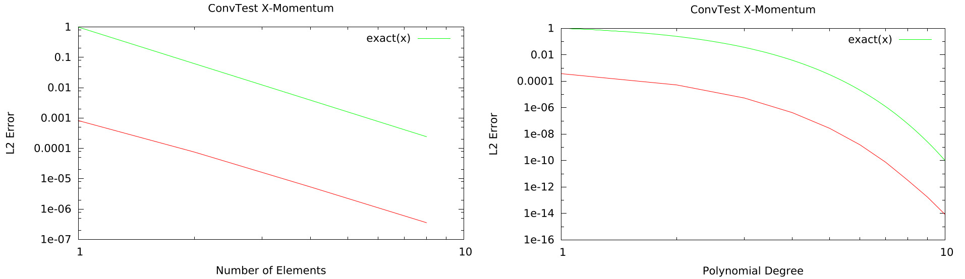
../../_images/convtest_result_plot.jpg — Fig. 5.5 Convergence test: Plot of spectral (right) and grid (left) convergence

5.3.4. Viscous Convergence Test

The second convergence test includes the viscous terms, i.e., convergence for the Navier-Stokes equations.

5.3.4.1. Manufactured Solution

For this case, another manufactured solution is chosen as

\[\rho = 2 + A*\sin(\Omega*|\underline{x}| - v\pi t) \quad \text{with} \quad A,\Omega,v = const.\]

The same function is applied to the momentum equations in all spatial directions. The mass specific total energy in this case is \(\rho e = \rho \rho\). Since the Navier–Stokes equations are considered, the manufactured solution has a non-zero source term. In FLEXI, this source term is added in the routine CalcSource in the file

src/equations/navierstokes/idealgas/exactfunc.f90

Note

This manufactured solution can also be solved without considering the viscous terms. In this case, the source term does not vanish.

5.3.4.2. Compiler Options

FLEXI should be compiled with the convtest_viscous preset using the following commands:

cmake -B build --preset convtest_viscous
cmake --build build

5.3.4.3. Simulation Parameters

The viscid convergence test is run from the parameter file parameter_convtestvisc_flexi.ini. The default settings for the viscous terms are displayed in Table 5.4.

Table 5.5 Numerical settings used for the viscid convtest.
Variable	Value	Description
IniExactFunc	4	The manufactured solution and the function used to initialize FLEXI. It can also be used for Dirichlet BCs.
Viscosity	0.03	Dynamic viscosity \(\mu_0\)

5.3.4.4. Simulation and Results

Execution of the viscous convergence tests is analogously to the inviscid case, e.g., with the following command.

tools/convergence_test/convergence_grid flexi parameter_convtestvisc_flexi.ini --gnuplot