5.10. Flow Around a NACA0012 Airfoil
In this tutorial, the simulation around a NACA0012 airfoil at \(Re = 5000\) and \(Ma = 0.4\) is considered. First, we explain how to set the main flow parameters. Next, we describe the evaluation of lift and drag and visualization of the flow field. Finally, we show how to use the sponge zone to remove artificial reflections from the outflow boundary, so that a clean acoustic field is retained. The tutorial is located at tutorials/naca0012.
5.10.1. Flow Description
A NACA0012 airfoil is placed in a semi-circular domain, extruded in the downstream direction. The chord length is normalized to 1 with an inflow velocity of \(1\) at an angle of attack (AoA) of \(8^\circ\). The viscosity and internal energy are scaled to obtain the desired Reynolds and Mach number, respectively. Fig. 5.29 displays the Mach number distribution along the domain centerline in the vicinity of the airfoil.
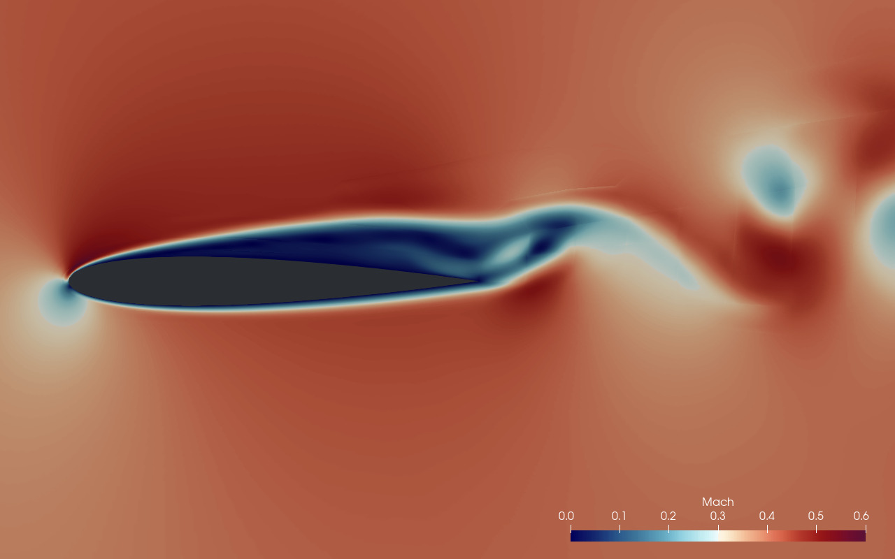
Fig. 5.29 Mach number distribution around the NACA0012 airfoil.
5.10.2. Mesh Generation
The mesh file used by FLEXI is created from the external linear mesh NACA0012_652.cgns and a 3rd-order boundary description NACA0012_652_splitNg2.cgns using HOPR. Obtain the executable and run the following command which creates the mesh file NACA0012_652_Ng2_mesh.h5 in HDF5 format.
hopr parameter_hopr.ini
5.10.3. Build Configuration
FLEXI should be compiled with the naca0012 preset using the following commands.
cmake -B build --preset naca0012
cmake --build build
5.10.4. Simulation Parameters
The simulation setup is defined in parameter_flexi.ini. The initial condition is selected via the variable vector RefState which represents the vector of primitive solution variables \((\rho, u, v, w, p)^T\).
5.10.4.1. Material Properties
! ============================================================ !
! Equation of State
! ============================================================ !
RefState          = (/1.,0.990268069,0.139173101,0.,4.4642857/)
IniExactFunc      = 1           ! Exact function for initial solution
IniRefState       = 1           ! Refstate used  for initial solution
kappa             = 1.4         ! Heat capacity ratio / isentropic exponent
R                 = 2.857142857 ! Specific gas constant
Pr                = 0.720       ! Prandtl number
mu0               = 0.0002      ! Dynamic Viscosity
The chosen velocity vector \((u,v)^T\) yields an angle of attack of \(\alpha=8^\circ\) and a velocity magnitude of \(1\). The RefState are numbered in the order they are supplied in the parameter file. Material properties are selected as described above. Based on the ideal gas law, we get
Note that in this non-dimensional setup, the mesh is scaled such that the chord length is unity, i.e., \(C=1\). Then, to arrive at \(Re=\rho u C / \mu = 5000\), the viscosity is set to
5.10.4.2. Numerical Setup
The DG method in FLEXI represents the solution on the mesh using piecewise polynomials. The polynomial degree in this tutorial is chosen as \(N=3\). The remaining numerical settings for the NACA0012 tutorial are summarized below.
N                 = 3        ! Polynomial degree
MeshFile          =  NACA0012_652_Ng2_mesh.h5
TEnd              = 10       ! End time of the simulation
Analyze_dt        = 0.01     ! Time interval for analysis
CFLscale          = 0.9      ! Scaling for the theoretical CFL number
DFLscale          = 0.9      ! Scaling for the theoretical DFL number
5.10.4.3. Boundary Conditions
Additionally, the setup requires the specification of the boundary conditions for all domain boundaries.
! ============================================================ !
! BOUNDARY CONDITIONS
! ============================================================ !
BoundaryName      = BC_wall
BoundaryType      = (/3,1/)     ! Adiabatic wall condition
BoundaryName      = BC_inflow
BoundaryType      = (/2,0/)     ! Weak Dirichlet condition
BoundaryName      = BC_outflow
BoundaryType      = (/2,0/)     ! Weak Dirichlet condition
BoundaryName      = BC_zminus
BoundaryType      = (/1,0/)     ! Periodicity condition
BoundaryName      = BC_zplus
BoundaryType      = (/1,0/)     ! Periodicity condition
The freestream boundaries are set to weak Dirichlet conditions (BCType=2) using the same reference state as the initialization. The airfoil boundaries are set to adiabatic walls (BCType=3). The boundary conditions in \(z\)-direction are not relevant for this quasi-2D example and are realized as periodic boundaries (BCType=1). All boundary conditions are summarized in the boundary conditions section.
5.10.5. Simulation and Results
We proceed by running the code in parallel. Here, <NUM_PROCS> is an integer denoting the number of processes to be used in parallel.
mpirun -np <NUM_PROCS> flexi parameter_flexi.ini
5.10.5.1. Lift and Drag Forces
The forces acting on the airfoil are one of the main desired output quantities from the simulation. They are calculated on the fly during runtime.
CalcBodyForces    = T           ! Compute body forces at walls
WriteBodyForces   = T           ! Write body forces to file
CalcBodyForces activates the integration of the pressure and viscous forces at each Analyze_dt. WriteBodyForces enforces output of the forces to a <PROJECTNAME>_BodyForces_<BOUNDARYNAME>.csv. In addition to being relevant to the airfoil performance, the body forces are a good measure for convergence. In the context of time-dependent flows, this determines whether the solution has reached a quasi-steady state. Fig. 5.30 shows the \(x\)- and \(y\)-components of the force acting on the airfoil until \(TEnd=10\). The lift and drag coefficients can be easily calculated by rotating these forces from the computational reference frame to the one of the freestream.
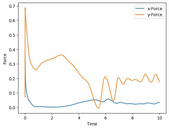
Fig. 5.30 Resulting forces on the NACA0012 airfoil.
From the forces, it is clear that the steady state has not yet been reached and the simulation must be run further. Before we proceed with the simulation, we will nonetheless examine the preliminary results to check the quality of the simulation.
5.10.5.2. Wall Velocities
Due to the weak coupling between the grid cells and to boundaries, boundary conditions are enforced weakly, e.g. by applying a specific flux. This adds largely to the stability of the scheme. However, as a result the no-slip condition at the wall is not exactly fulfilled by the numerical solution. Rather, it is approximated as far as the resolution allows. Evaluation of the velocity vector near the wall helps quantifying this error, which can be seen as a quality measure for the near wall resolution.
CalcWallVelocity  = T           ! Compute velocities at wall boundaries
WriteBodyForces   = T           ! Write wall velocities to file
CalcWallVelocity activates the integration of the wall velocities at each Analyze_dt. WriteWallVelocity enforces output of the wall velocities to a <PROJECTNAME>_WallVel_<BOUNDARYNAME>.csv.
During the computation, we get output like the following.
 Wall Velocities (mean/min/max)  :
       BC_wall   2.661973831E-02   2.303391807E-04   6.206912250E-01
In our case, the wall velocity is on average at about \(3\%\) of the freestream velocity, reaching a peak of \(60\%\). This peak typically occurs at the quasi-singularity at the trailing edge. To decrease this deviation from the theoretical no-slip condition, either the wall-normal mesh size must be decreased or the polynomial degree increased. It is important to note that both of these measures will, besides increasing the number of degrees of freedom, decrease the time step, which directly affects the computational time. Thus, it is important to achieve an acceptable trade-off between the acceptable error and the computational time. In this tutorial, the observed slip velocity is deemed uncritical and we proceed with the same resolution.
5.10.5.3. Visualization
FLEXI relies on ParaView for its visualization. To visualize the FLEXI solution, it must be converted from the HDF5 format into a format suitable for Paraview. FLEXI provides a post-processing tool posti_visu which generates files in VTK format when running the following command.
mpirun -np 4 posti_visu parameter_postiVisu.ini parameter_flexi.ini NACA0012_Re5000_AoA8_State_0000000.0*
Fig. 5.31 shows a visualization of the density distribution at \(t=10\). The large scale vortex shedding of the wake due to the high angle of attack is clearly visible. Acoustic radiation from the airfoil can also be observed. Now, a problem becomes apparent: the vortex street propagating towards the outflow boundary results in a second, artificial acoustic source at the outflow boundary. This is one of the fundamental problems in direct aeroacoustic computations. Before we proceed with the simulation, we will now make use of the sponge zone functionality of FLEXI to remove this artificial source.
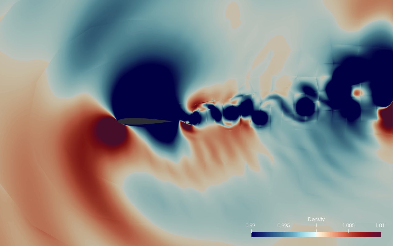
Fig. 5.31 Density field around the NACA0012 airfoil.
5.10.5.4. Sponge Zone
The sponge zone introduces a dissipative source term to the discrete operator, which is only active in a user-specified region, typically upstream of the outflow boundary. We use the sponge zone to dampen the vortices convected downstream before they hit the outflow boundary. The associated flags in the parameter file are given in SPONGE section of the parameter_flexi.ini file. See [8] for the background of our sponge zone implementation.
! ============================================================ !
! SPONGE
! ============================================================ !
SpongeLayer           = T           ! Enables the dissipative source term
SpongeShape           = 1           ! Shape of sponge: 1: Cartesian
damping               = 1.0         ! Damping factor of sponge
SpongeXStart          = (/2.0,0,0/) ! Coordinates of start position of sponge
                                    ! - ramp (for SpongeShape=1)
SpongeDistance        = 3.0         ! Length of the sponge ramp
                                    ! - ramp (for SpongeShape=1)
SpongeDir             = (/1,0,0/)   ! Direction vector of the sponge ramp
                                    ! - ramp (for SpongeShape=1)
SpongeBaseFlow        = 4           ! Type of baseflow to be used for sponge
                                    ! - 4: moving average (Pruett baseflow)
tempFilterWidthSponge = 2.0         ! Temporal filter width used to advance
                                    ! Pruett baseflow in time
SpongeViz             = T           ! Write a visualization file of the sponge strength
The source term is of the form
First, damping determines the strength of the source term, i.e., \(d\) in eq. (5.3). It is dependent on the mean convection velocity, the desired amount of amplitude reduction and, the thickness of the sponge zone. Typically, some trial and error is necessary to obtain an appropriate value. In non-dimensional calculations, i.e., velocity and length scale are of \(\mathcal{O}(1)\), \(d=0.1 \ldots 2\).
Ramping of the source term from \(0\) is necessary to avoid reflections at the sponge interface. If such reflections occur, it is necessary to choose a wider sponge ramp, so that the source term is ramped up more gradually. We choose a parallel ramp by setting SpongeShape=1. The ramp’s start position, thickness, and direction are controlled by the parameters SpongeXStart, SpongeDistance and SpongeDir, respectively. These parameters govern the shape function \(\sigma(\vec{x})\) which smoothly ramps the source term from \(0\) to \(1\). With the chosen settings, the sponge zone starts one chord behind the airfoil and is ramped up to \(1\) at the outflow boundary, located \(4\) chords behind the airfoil. In order to visualize the ramping function \(d\sigma(\vec{x})\), set SpongeViz=T.
Caution
The sponge zone is not a physical region but a boundary condition. Place the active source regions far enough downstream of the airfoil to ensure they do not influence the near-field solution.
Next, select the desired base flow, (\(U_B\)). For the current configuration, the moving average (SpongeBaseFlow=4) is appropriate. It produces a mean field slowly progressing in time, which adapts to the airfoil’s surrounding flow. The parameter tempFilterWidthSponge determines the effective time window for this average and should be set slightly longer than the largest time scales to be damped. In this example, we use tempFilterWidthSponge=2.0, chosen based on the frequency of oscillations in the body forces, as shown in Fig. 5.30.
The moving average base flow requires an initial field. One option is to provide an initial flow field from a file using the SpongeRefFile parameter. If this parameter is not set, If this parameter is not set, the code initializes the base flow with the current solution field. Therefore:
For a new simulation, the base flow is initialized with
IniExactFunc, which also initializes the solution.For a restarted simulation, as in this example, the base flow is initialized using the state file provided for the restart.
Important
When using the moving average base flow, the code creates *baseflow*.h5 files for restarting with the saved base flow state. If these files match the current project name, they are automatically loaded. However, if SpongeRefFile is also specified, the base flow restarts from that file instead, which may unintentionally reset the flow state.
5.10.6. Restarting the Simulation
If the simulation is interrupted or needs to extend beyond TEnd=10, FLEXI can be restarted easily. With the current settings, the solution is saved every \(0.1\) time units, so to continue the simulation, update TEnd=25 in the parameter file. Since we have now turned on the sponge zone, it is also advisable to modify the project name, i.e.
ProjectName = NACA0012_Re5000_AoA8_SP
To restart the simulation, ensure the state files are in the current folder, then run
mpirun -np 4 flexi parameter_flexi.ini NACA0012_Re5000_AoA8_State_0000010.000000000.h5
You can also adjust the polynomial degree N during restart, allowing a lower initial degree for faster convergence, then a higher degree for improved accuracy. The code will automatically project the solution onto the new polynomial basis at startup, but restart is only possible with the same mesh file.
5.10.7. Two-dimensional Computation
The laminar flow around this airfoil is inherently two-dimensional. However, so for this simulation was run using a three-dimensional code by imposing periodic boundary conditions with only one mesh element in the spanwise direction. This means we
Compute one unnecessary variable (momentum in spanwise direction),
Compute three-dimensional fluxes for all variables,
Compute one unnecessary gradient,
Use several degrees of freedom in the spanwise direction due to the high order ansatz in each element.
To avoid these inefficiencies, FLEXI provides an option for true two-dimensional calculations. Set the flag FLEXI_2D=ON during configuration, which enables two-dimensional mode. Navigate to your build directory, set the FLEXI_2D flag in CMake, reconfigure, and recompile. You must also use a mesh with only one element in the third dimension. Since the tutorial mesh meets this requirement, you can start two-dimensional calculations immediately after recompiling with FLEXI_2D enabled.
Once compiled, you can rerun the code with the same parameter file using the new executable. All settings for two-dimensional and three-dimensional computations remain the same. For compatibility, vector parameters (like momentum in RefState) should still specify three dimensions; however, the third dimension will simply be ignored. Pay attention to how much faster your code runs when using the two-dimensional version.
By default, FLEXI saves State files in a three-dimensional format by extruding the solution, ensuring compatibility with existing post-processing tools. To save space, you can set Output2D=T to write two-dimensional files. Note that, regardless of dimensionality, arrays retain three dimensions (with one dimension of size 1 for two-dimensional simulations), and all variables, including the spanwise momentum, are still present but set to zero without performing calculations.
5.10.8. Record Points (Probes)
To track the evolution of flow variables near the airfoil’s upper and lower surfaces, recording the entire flow field in State files can be costly, especially for high temporal resolution or large fields. FLEXI offers record points (commonly also known as probes) to sample specific flow locations at high temporal resolutions (even down to a single time step) to reduce storage costs.
Setting up record points involves three steps
Creating the record points
Running a simulation with active record points
Visualizing the results
The first and third steps are performed with pre- and post-processing tools, respectively. Enabling record points in a simulation just requires setting the respective options in FLEXI.
5.10.8.1. Record Points Preparation
The coordinates of the record points are defined using the POSTI tool preparerecordpoints, which is built when the corresponding CMake option is enabled. The tool takes a single parameter file as an input, so run it as follows:
posti_preparerecordpoints parameter_recordpoints.ini
A sample parameter file is included in the NACA0012 tutorial folder. Define the mesh and project name in this file. The options NSuper and maxTolerance adjust the record point search algorithm; setting NSuper to at least twice the mesh’s polynomial degree is a good starting point. The remainder of the parameter file is the actual definition of the record points.
Record points are organized in sets, with each set a part of a named group. In the example, two sets are created - one for the suction and one for the pressure side of the airfoil -, each assigned to a separate group. FLEXI supports several differing set types, such as single points, lines, or planes. For the NACA example, we use the boundary layer plane set type. This set defines a special type of plane by projecting a spline onto the nearest boundary and distributing a user-specified number of points along this line. The plane is then created through extrusion along the boundary’s normal vector over a specified distance, with optional stretching to cluster points near the wall. The definition of one of the groups looks like this:
GroupName           = suctionSide
BLPlane_GroupID     = 1
BLPlane_nRP         = (/20,30/)
BLPlane_nCP         = 2
BLPlane_CP          = (/0.9,0.014,0.5/)
BLPlane_height      = 0.05
BLPlane_CP          = (/0.999,0.001,0.5/)
BLPlane_height      = 0.05
BLPlane_fac         = 1.04
Each set of record points must be assigned to a group for identification purposes. The assignment is specified with the GroupID (e.g., BLPlane_GroupID), here set to \(1\) for assignment to the first group. After defining the group, configure the parameters of the set. For a boundary layer plane, set the number of points along wall-tangential and wall-normal directions using BLPlane_nRP. Then, specify the spline projected onto the boundary. Set the number of control points in the boundary (BLPlane_nCP), the coordinates of each control point (BLPlane_CP), the height in the wall-normal direction at this point (BLPlane_height) and the stretching factor applied in the wall-normal direction (BLPlane_fac). For details on defining other set types, refer to their respective parameter descriptions.
When you run the preparerecordpoints tool, it computes the physical coordinates of the record points based on your definitions. The tool then identifies the mesh elements containing each record point and calculates the coordinates in the reference element using Newton’s method for interpolation. The results are saved in a file named <PROJECTNAME>_RPSet.h5. If you enable the doVisuRP option, a visualization of the record points is generated for viewing in ParaView.
5.10.8.2. Record Points Usage
To utilize record points during a simulation, simply set a few options in the FLEXI parameter file. The essential options are given in the following.
RP_inUse            = T
RP_DefFile          = NACA0012_RPSet.h5
RP_SamplingOffset   = 1
With the RP_inUse option, the record points system is enabled or disabled. The RP_DefFile option specifies the name of the file created by the preparerecordpoints tool containing the record points definitions (e.g., NACA0012_RPSet.h5). The RP_SamplingOffset option determines the sampling interval for the solution, allowing you to specify that the solution should be sampled at every RP_SamplingOffset timestep.
When you run the simulation, in addition to the State files, corresponding RP files are generated, containing the conservative variable values at each record point for every sampling timestep.
5.10.8.3. Record Points Post-Processing
Record points data is post-processed using the visualizerecordpoints tool. It can merge multiple RPSet.h5 files to create an extended time series. In addition to visualizing the time series, a multitude of post-processing options is available. These options allow you to compute the mean and fluctuating components of the solution or perform spectral analysis using FFTs. For boundary layer planes, different turbulent quantities, such as skin friction, can be computed directly.
For example, we want to calculate the mean flow \(\bar{U}\) and the temporal fluctuations \(U\)) at our two record point planes. A sample parameter file for the tool is provided in the tutorial folder. The options set in the parameter file are
ProjectName         = NACA0012
RP_DefFile          = NACA0012_RPSet.h5
GroupName           = suctionSide
GroupName           = pressureSide
OutputTimeAverage   = T
doFluctuations      = T
In this configuration, we specify a name for the project (ProjectName) and provide the path to the file containing the record point definitions (RP_DefFile). The GroupName options correspond to the names we defined while using the preparerecordpoints tool. To evaluate the data, we calculate the temporal average and the fluctuations, which are determined using the equation
We did not specify any specific variables for visualization, meaning all conservative variables stored in the RPSet.h5 files will be utilized. If you wish to visualize a specific or derived variable (e.g., pressure), you can simply set it in the parameter file as follows
VarName = Pressure
You can execute the tool using the command
posti_visualizerecordpoints parameter_visualizeRecordpoints.ini NACA0012_Re5000_AoA8_RP_*
This takes all the time samples recorded during the simulation as input. For each of the planes, a separate .vts file containing the temporal average is generated. The fluctuations are time-resolved data, and due to limitations in the VTK file format, each time step must be written to a single file. To prevent the creation of numerous files in the working directory, these files can be organized into a subfolder named timeseries. In this case, .pvd files for the fluctuations are created in the working directory. These files can be opened with ParaView, containing the complete time series along with the correct time values. If you to not require ParaView compatibility, the complete solution can be written in a single HDF5 file by setting
OutputFormat = HDF5