5.9. Flow Around a Cylinder
In this tutorial, the simulation around a two-dimensional circular cylinder at \(Re_D=200\) and \(Ma=0.2\) is considered. The goal of this tutorial is to introduce the usage of temporal probes, here called “record points”, together with the associated posti_visualizerecordpoints tool. Furthermore, we introduce the posti_dmd tool and use it for dynamic mode decomposition (DMD). This tutorial is located in the folder tutorials/cylinder.
5.9.1. Flow Description
The setup considered consists of a 2D rectangular domain with the primary flow in \(x\)-direction, from left to right. Being a 2D plane, it corresponds to the “look-down” view upon the domain and the cylinder. The imposed flow is sufficiently fast for the wake of the cylinder to turn from a laminar flow to a street of shed vortices. It is the goal of the dynamic mode decomposition to analyze the primary oscillation frequencies present in these shed vortices.
5.9.2. Build Configuration
FLEXI should be compiled with the cylinder preset using the following commands.
cmake -B build --preset cylinder
cmake --build build
5.9.3. Mesh Generation
We use a curved mesh with \(1000\) cells for the tutorial. The mesh is deformed to align with the cylinder boundary in the center. Furthermore, we utilize stretching in wall-normal direction to increase the resolution in the crucial near-wall region and relax it towards the domain boundaries. In case you want to generate other meshes, the parameter file for HOPR is included in the tutorial directory as parameter_hopr.ini.
5.9.4. Simulation Parameters
The simulation setup is defined in parameter_flexi.ini. The initial condition is selected via the variable vector RefState=(/1.,1.0,0.,0.,17.857/) which represents the vector of primitive solution variables \((\rho, u, v, w, p)^T\).
5.9.4.1. Material Properties
The material properties of the considered fluid are defined in the equation of state section. We chose the Prandtl number \(Pr\) and the isentropic coefficient \(\kappa\) to their default values of \(Pr = 0.72\) and \(\kappa = 1.4\), respectively. Thus, they are omitted in the parameter file.
! ============================================================ !
! Equation of State
! ============================================================ !
R                 = 17.857   ! ideal gas constant
Mu0               = 0.005    ! dynamic viscosity
Based on the ideal gas law, we get
Note that in this non-dimensional setup the mesh is scaled such that the reference length is unity, i.e., \(D=1\). Then to arrive at \(Re=\rho u D / \mu = 200\), the viscosity is set to
5.9.4.2. Boundary Conditions
The boundary conditions were already set in the mesh file by HOPR. Thus, the simulation runs without specifying the boundary conditions in the FLEXI parameter file. The freestream boundaries of the mesh are Dirichlet boundaries using the same state as the initialization, the wall is modeled as an adiabatic wall. The boundary conditions in \(z\) direction are not relevant for this 2D example, but would be realized as periodic boundaries for a 3D simulation.
5.9.5. Simulation and Results
We proceed by running the code with the following command.
flexi parameter_flexi.ini
If FLEXI was compiled with MPI support, it can also be run in parallel with the following command. Here, <NUM_PROCS> is an integer denoting the number of processes to be used in parallel.
mpirun -np <NUM_PROCS> flexi parameter_flexi.ini
The simulation runs for 300 convective time units to achieve periodic vortex shedding, thus - depending on your machine - the simulation can take up to one to two hours.
5.9.5.1. Evaluation of the Strouhal Number
The Strouhal number (which is a non-dimensional frequency, \(Sr=\frac{f \cdot D}{u}\), describing the oscillatory motion of the flow) is estimated using the forces acting on the cylinder induced by the vortex shedding. The forces are calculated on the fly during runtime. The associated flags in the parameter file are the following.
CalcBodyForces    = T        ! Calculate body forces (BC 4/9)
WriteBodyForces   = T
The first line activates the calculation of the forces at each Analyze_dt, the second line enforces output of the forces to a file. In Fig. 5.26 the force in y-direction is plotted. By measuring the time from peak to peak over several periods the Strouhal number can be estimated to \(0.1959\) which is close to the expected value from literature.
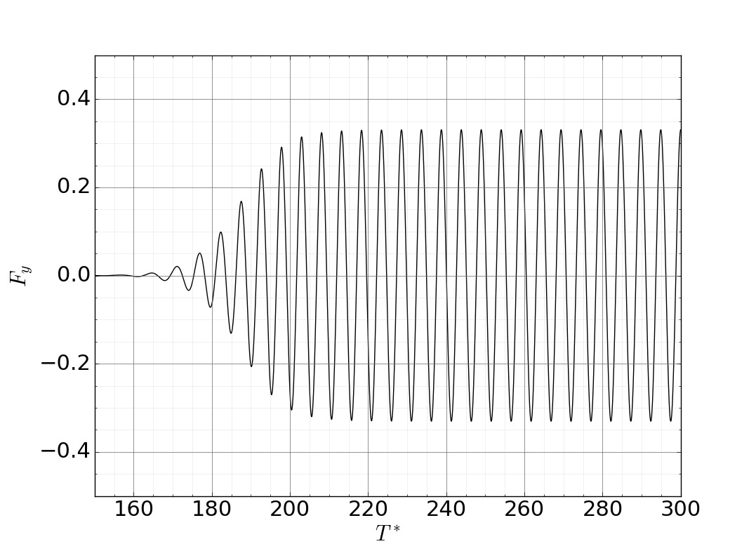
Fig. 5.26 Resulting lift forces on the cylinder.
5.9.5.2. Evaluation of the Separation Angle
The mean separation angle is evaluated using the record point tool as described in Recordpoints. The simulation setup already contains the record points set and output of the record points during the simulation is enabled by the default parameter file. The record points set contains probes distributed along a plane within the boundary layer of the upper cylinder side. For the calculation of the separation angle, we want to use the Plane_doBLProps functionality within the posti_visualizerecordpoints tool. In addition to the namesake visualization functionality, this tool has options to analyze the boundary layer properties such as the wall friction to estimate the separation point. The required parameters are already set in the parameter_visualizeRecordpoints.ini file. Thus, you can directly invoke the tool by running the following command.
posti_visualizerecordpoints parameter_visualizeRecordpoints.ini Cylinder_Re200_RP_*
After executing the tool, you will get a file named Cylinder_RP_BLProps_upperSide_BLPla000001.vts which can be visualized with ParaView. Since the data were are interested in is one-dimensional, you won’t be able
to see the data in the default render view. Instead, choose the Plot Over Line filter and ParaView should automatically apply the correct plot range. As separation occurs when the skin friction falls to zero, you can estimate the separation angle to \(110^{\circ}\) by plotting tau_w over the circumference and finding the intersection with the \(y=0\) axis.
5.9.6. Dynamic Mode Decomposition
The dynamic mode decomposition (DMD) is an algorithm to divide a temporal series into a set of modes which are associated with a frequency and growth/decay rate. Thus, DMD allows us to determine temporal dependencies such as the Strouhal frequency. The DMD in FLEXI is implemented according to Schmid et al. [28] and available through the posti tool posti_dmd.
As the DMD operates in the frequency domain, we need a higher temporal resolution of the written state files. Thus, change the time TEnd to \(310\) and nWriteData to \(1\). Then, restart the FLEXI simulation from the latest state file with the following command.
flexi parameter_flexi.ini Cylinder_Re200_State_0000300.000000000.h5
Once the simulation concludes, execute the DMD on the generated state files. The parameter_dmd.ini is pre-configured to perform a DMD on the density, thus we can invoke the following command.
posti_dmd parameter_dmd.ini Cylinder_Re200_State_00003*
Attention
Dynamic Mode Decomposition (DMD) is performed in the frequency domain and requires the complete solution to be loaded into memory. Depending on the available memory, you might have to decrease the number of input state files.
During execution, two additional files Cylinder_Re200_DMD_0000300.000000000.h5 and Cylinder_Re200_DMD_Spec_0000300.000000000.dat are generated. The first file contains a field representation of the different modes, the
second file contains the Ritz spectrum of the modes. Thus, the field can be visualized in ParaView after conversion to VTK format with the following command.
posti_visu parameter_postivisuDMD.ini Cylinder_Re200_DMD_0000300.000000000.h5
The new file Cylinder_Re200_Solution_0000300.000000000.vtu now contains four modes available for visualization. Fig. 5.27 shows the global, the first, the second, and the third harmonic mode. The first mode is the mode of the considered Strouhal number.
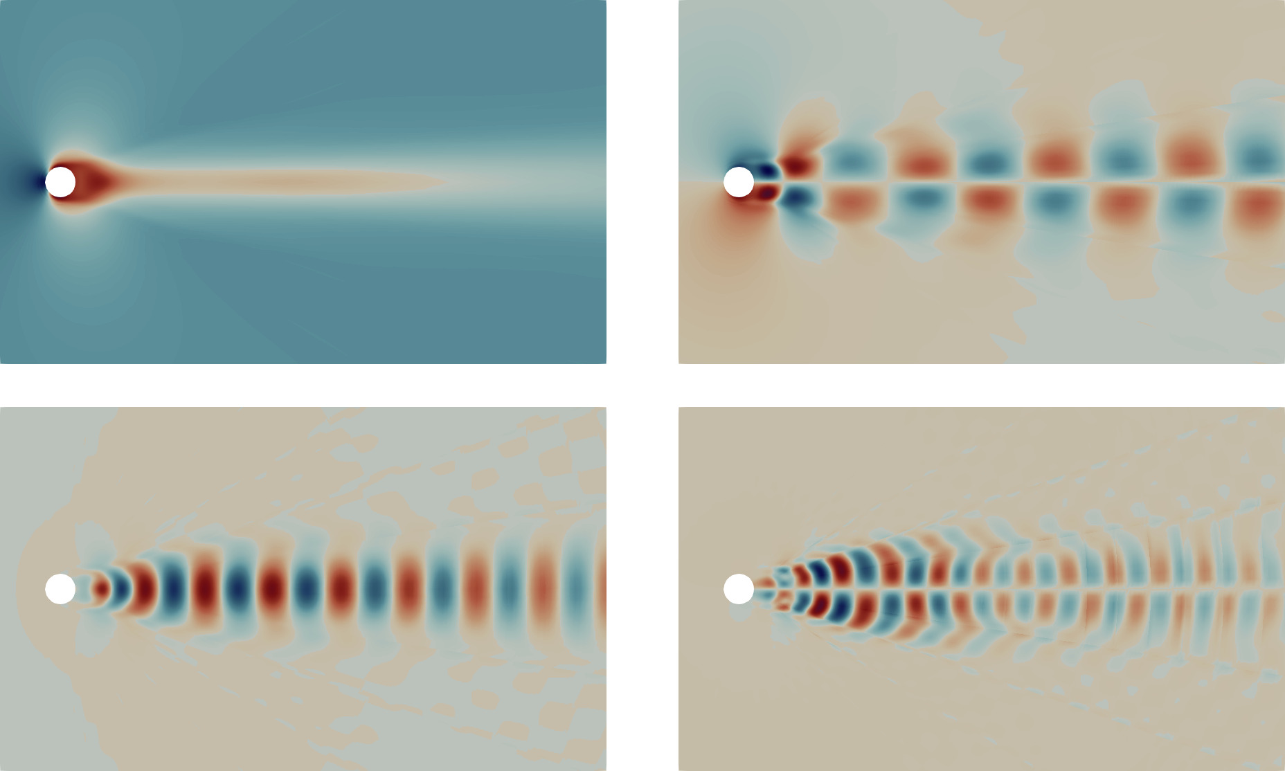
Fig. 5.27 DMD modes of the density field. Top left global mode, top right first harmonic, bottom left second harmonic, bottom right third harmonic.
The Ritz spectrum in DMD is a set of complex numbers that represent the eigenvalues of a low-rank approximation of the Koopman operator. These eigenvalues provide information about the frequencies and growth rates of the dominant modes present in the flow data. FLEXI contains a Python script tools/plot_RitzSpectrum.py which we can execute on the DMD data file to obtain the Ritz spectrum.
python plot_RitzSpectrum.py -d Cylinder_Re200_DMD_Spec_0000300.000000000.dat
The result is a Ritz spectrum as shown in Fig. 5.28. Here, the abscissa shows the frequency of the modes and the ordinate the growth/decay factor. Modes with \(\omega_r<0\) are damped. The modes placed directly on the abscissa are the already discussed modes, from left to right the global, the first, the second harmonic mode and so on. The color and size of the modes represent the Euclidean norm of the mode which can be interpreted as an energy norm of the mode.
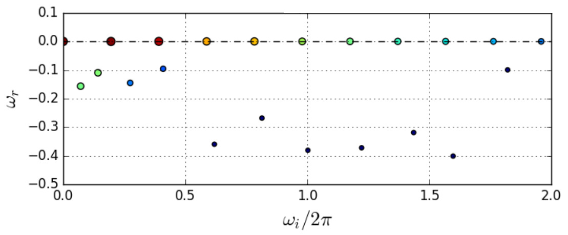
Fig. 5.28 Ritz spectrum.