4. Workflow

This chapter describes the complete process of performing a simulation in FLEXI. The process comprises the mesh generation using the high-order pre-processor HOPR, the actual simulation of the numerical problem, and the post-processing step using the POSTI toolchain. An overview of this workflow and the components of FLEXI is given in the flowchart below.

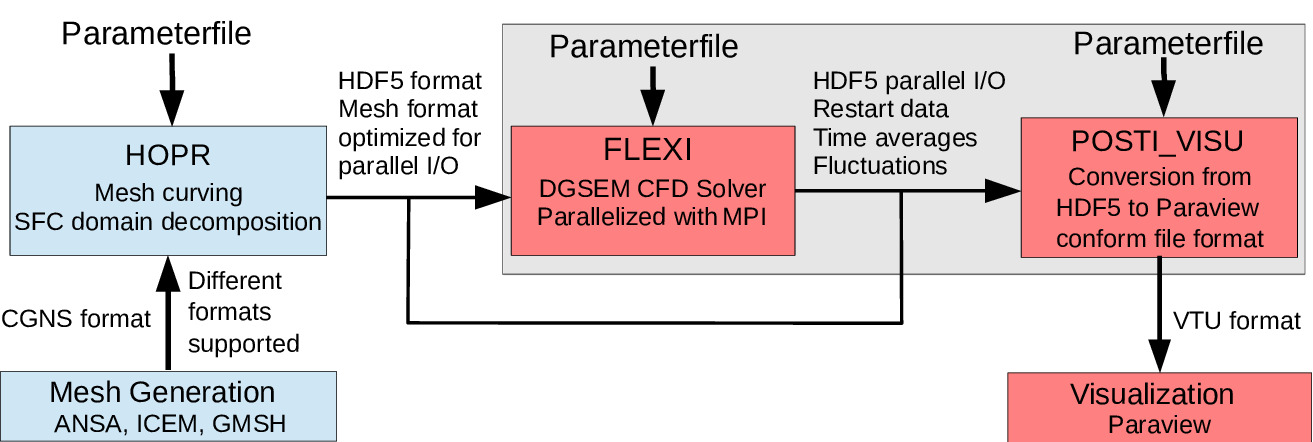
Basic modules and files used by FLEXI. — Fig. 4.1 Basic modules and files used by **FLEXI**.

Note that both, HOPR and FLEXI, use the HDF5 format to output mesh files and simulation states, respectively. HDF5 is a widely used data model, library, and file format for storing and managing data. It supports an unlimited variety of data types, and is designed for flexible and efficient I/O, and for high volume, complex data. We refer to the HDF5 website for further information on this file format in general.

4.1. Mesh Generation using HOPR

FLEXI obtains its computational meshes from the high-order preprocessor HOPR (available under GPLv3 at HOPR project) in HDF5 format. The design philosophy is that all tasks related to mesh organization, different input formats and the construction of high-order geometric mappings are separated from the parallel simulation code. The serial standalone framework HOPR has been developed to generate high-order meshes from input data by external linear mesh generators, supporting different file formats. It also provides a built-in mesh generator for simple, structured meshes. HOPR can either be compiled from the source code or be used directly via the provided AppImage, both available on its github page.

The basic command to run HOPR is

hopr parameter_hopr.ini

where the path to the HOPR executable has been omitted for simplicity. The test cases provided in chapter Tutorials come with both a ready-to-use mesh file and a parameter file for HOPR, which can be used to generate or modify the meshes as needed. Provided the mesh file has been set up, its location must be specified in the FLEXI parameter file.

MeshFile=path/to/mesh/file.h5

4.2. Build Configuration

Before setting up a simulation, the code must be compiled in the desired configuration. An overview of the most commonly used compiler options is given in section Compiler Options. The default configuration solves the three-dimensional Navier–Stokes equations using the pure DG operator (no FV shock-capturing) and does not compile any POSTI tools.

4.2.1. Using CMake Presets

The build configurations used for the Tutorials are stored as CMake presets (human-readable format) in CMakePresets.json located in the FLEXI root directory. They can be applied by creating a build folder, reading the desired preset and compiling the code:

mkdir build
cmake -B build --preset <preset_name>
cmake --build build

Caution

CMake presets were introduced in CMake version 3.19. For earlier versions, FLEXI can only be configured manually.

4.2.2. Manual Configuration

To configure the code manually, you can use the CMake GUI, which displays brief instructions and descriptions of the compiler options at the bottom of the window. Note that some compiler options are dependent on others, such that you should always configure by hitting the c key after changing the value of a compile option. In order to change values, use the arrow keys to select a compile option, and hit the enter key to edit its value; boolean options will toggle with the enter key. Once all desired options are set, generate the Makefiles by hitting the g key, exit by hitting the q key and compile using make:

mkdir build
ccmake -B build
cmake --build build

4.3. Parameter File

The computational setup of the considered test case, including solver settings, initial, and boundary conditions, material properties, data output, is specified via a parameter file. This file is typically named parameter_flexi_ini and contains a simple list of parameters, given in the form

! This is a comment, e.g. section heading
parameter_name = parameter_value

Note that the format is case-insensitive (Fortran-style) and that some parameters can also be listed multiple times (so-called CountOptions).

To get a list and short description of all possible parameters, grouped thematically, run the FLEXI help

flexi --help

To confine the output to the parameters of a certain section or only one specific parameter, respectively, run

flexi --help SECTION
flexi --help PARAMETER

4.3.1. Solver Settings

The definition of the numerical solver typically covers the following steps.

Set the polynomial degree.

Define the polynomial degree N of the solution. The order of convergence follows as \(N+1\). Each grid cell contains \((N+1)^3\) collocation points to represent the solution.
Choose a dealiasing approach.

For under-resolved Navier-Stokes simulations, e.g., in an LES setting, dealiasing is important for numerical stability. Various choices are available and set using either over-integration or a split-form DG scheme. As the performance penalty of over-integration is substantial, the usage of the split formulation is recommended.
- OverintegrationType=1 is a filtering strategy, where the complete operator is first evaluated at N (\(U_t^{N}\)) and then filtered to a lower effective degree NUnder (\(U_t^{Nunder}\)). To use this variant, specify Nunder to a value smaller than N.
- OverintegrationType=2 is a filtering strategy, where the operator in reference space, e.g., \(JU_t\), is first projected to the NUnder node set before converting it to physical space \(U^{Nunder}_t=JU^{Nunder}_t/J^{Nunder}\). This implementation enforces conservation. To use this variant, specify Nunder to a value smaller than N.
- SplitDG uses a split formulation, requiring the compiler option FLEXI_SPLIT_DG to be turned on. The most commonly used options are the kinetic energy stable formulation by Pirozzoli [14] (PI), the entropy conservative formulation by Chandrashekar [15] (CH) and a flux differencing form equivalent to the standard DGSEM (SD).
Choose a Riemann solver.

The Riemann solver defines how the inter-element coupling is accomplished. The available variants are listed in section Parameter File. Use the Riemann and the RiemannBC options to specify which Riemann solver is to be used at internal interfaces and at Dirichlet boundary conditions, respectively. The default Riemann solver is RoeEntropyFix.
Choose a time discretization method.

The time discretization method is set using the option TimeDiscMethod. Various explicit Runge-Kutta variants are available and listed in section Parameter File. By default, the low-storage fourth order Runge-Kutta scheme by [5] is employed.

4.3.2. Initial Conditions

Both initial and boundary conditions are controlled via the so-called RefState and ExactFunction constructs.

The RefState specifies a state vector in primitive form \((\rho,u,v,w,p)^\intercal\). An arbitrary number of reference states can be defined:

RefState=(/1,1,0,0,0.71428571/)
RefState=(/1,0.3,0,0,0.71428571/)

In this example, the first state describes a parallel flow in \(x\) direction at \(Ma=1\), the second state at \(Ma=0.3\), if an ideal gas with \(\kappa = 1.4\) is used.

The code contains a number of predefined analytic solution fields (ExactFunction), which are invoked by specifying their respective number. For instance, the initialization of a simple constant freestream is achieved by setting

IniExactFunc=1

The associated state vector to be used is determined by

IniRefState=1

which, in the above example would imply that the first RefState is used for initialization.

Note

The implemented exact functions are specific to the equation system and not documented comprehensively. They can be looked up in the source code, for example in src/equations/navierstokes/idealgas/exactfunc.f90.

4.3.3. Boundary Conditions

The names of the boundaries are contained in the mesh file and can be used in the FLEXI parameter file to override the boundary conditions set in the HOPR parameter file, if necessary.

FLEXI lists the boundaries and their respective boundary conditions during initialization, for example:

|                Name      Type     State     Alpha
|       BC_periodicz-         1         0         3
|       BC_periodicy-         1         0         2
|       BC_periodicx+         1         0        -1
|       BC_periodicy+         1         0        -2
|       BC_periodicx-         1         0         1
|       BC_periodicz+         1         0        -3

If we wished to apply a Dirichlet boundary condition with RefState=2 at the two boundaries in \(y\)-direction, we would have to add the following lines to the parameter file

BoundaryName=BC_periodicy-
BoundaryType=(/2,2/)
BoundaryName=BC_periodicy+
BoundaryType=(/2,2/)

Note that the first entry in the brackets specifies BC_TYPE, while the second specifies BC_STATE, in this case the number of the RefState to be used. In general, BC_STATE identifies either a RefState, an ExactFunction or remains empty, depending on the BC_TYPE.

The currently implemented boundary conditions for the Navier-Stokes equations are listed in the table below. See [9] for details on the listed inflow/outflow boundary conditions.

Table 4.1 Boundary conditions.
Boundary Condition	BC_TYPE	BC_STATE	Comment
Periodic BC	1	\(-\)	Can only be defined in HOPR
Weak Dirichlet	2	`RefState`
Weak Dirichlet	12	\(-\)	Like 2, but using an external state set by `BCStateFile`
Weak Dirichlet	22	`ExactFunction`	Like 2, but using an `ExactFunction`
Wall adiabatic	3	\(-\)
Wall isothermal	4	`RefState`	Isothermal wall, temperature is specified via \(p\) and \(\rho\) contained in the `RefState`
Wall slip	9	\(-\)	Slip, symmetry or Euler wall
Outflow Mach number	23	`RefState`
Outflow Pressure	24	`RefState`
Outflow Subsonic	25	`RefState`
Inflow total pressure / temperature	27	`RefState`	Special Refstate: total quantities \((T_t,\alpha,\beta,0,p_t)\)

4.3.4. Material Properties

At present, the only available equation of state in the Navier-Stokes solver of FLEXI is the ideal gas,

\[p = \rho R T\]

with the gas constant \(R\). The heat flux follows Fourier’s law

\[\vec{q} = -\lambda \nabla T \qquad \text{with} \quad \lambda = \frac{\kappa R \mu}{(\kappa-1) \mathrm{Pr}}\]

where \(\lambda\) denotes the heat capacity ratio, \(\mathrm{Pr}\) the Prandtl number and \(\mu\) the dynamic viscosity.

These parameters are specified in the parameter file using R, kappa, Pr and mu0, respectively.

4.3.5. Data Output

The end time of the simulation is set using tEnd. FLEXI features several analyze routines, which evaluate the current solution and are invoked every time interval Analyze_dt.

Specifically, the following evaluations are possible:

CalcErrorNorms=T: Calculate the \(L_2\) and \(L_\infty\) error norms based on the specified ExactFunc as reference. This evaluation is used for, e.g., convergence tests.
CalcBodyForces=T: Calculate the pressure and viscous forces acting on every wall boundary condition (BC_TYPE=3,4 or 9) separately. The forces are written to dat files.
CalcBulkState=T: Calculate the bulk quantities, such as the bulk velocity for the channel flow.
CalcWallVelocity=T: Due to the discontinuous solution space and the weakly enforced boundaries, the no-slip condition is not exactly fulfilled. The deviation depends mainly on the resolution in the near-wall region. Thus, this evaluation can be used as a resolution measure at the wall.

The solution itself is dumped to hard drive every Analyze_dt as well, unless a multiple of this time interval is specified via nWriteData. For example, nWriteData=10 means that the solution output is performed every tenth analyze time step only.

4.4. Running the Simulation

In general, the simulation is started by running

flexi parameter.ini [restart_file.h5]

The restart file is optional and allows resuming the simulation from any existing state file.

Attention

When restarting from an earlier time (or zero), all later state file possibly located in the present directory are deleted!

The simulation code is specifically designed for (massively) parallel execution using the MPI library. For parallel runs, the code must be compiled with LIBS_USE_MPI=ON. Parallel execution is then controlled using mpirun

mpirun -np <no. processors> flexi parameter.ini [restart_file.h5]

4.4.1. Domain Decomposition

The grid elements are organized along a space-filling curve (SFC), which gives a unique one-dimensional element list. The SFC type is controlled by HOPR, with the Hilbert curve set as default. In a parallel run, the mesh is partitioned into as many subdomains as deployed processors simply by splitting the SFC evenly. Thus, domain decomposition is done fully automatic and is not limited by, e.g., an integer factor between the number of cores and elements. The only limitation is that the number of cores must not exceed the number of mesh elements.

4.4.2. Choosing the Number of Cores

Parallel performance heavily depends on the number of processing cores. The performance index is defined as

\[PID=\frac{WallTime \times \#Cores}{\#DOF \times \#TimeSteps \times \#RKstages}\]

and measures the wall time per degree of freedom and stage of the time integration scheme. During runtime, the average \(PID\) is displayed in the output as

CALCULATION TIME PER STAGE/DOF: [ 5.59330E-07 sec ]

When compared to the single-core performance, it can be used as a parallel efficiency metric. The \(PID\) mainly depends on the processor workload

\[Load=\frac{\#DOF}{\#Cores}\]

and the polynomial degree \(N\). Processor workloads for optimal performance lie in the range \(Load=2000-5000\). A recent performance analysis on the HPE Appollo System HAWK using AMD EPYC 7742 CPUs is given in [16]

4.5. Test Case Environment

The test case environment can be used as to add test case-specific code for, e.g., custom source terms or diagnostics to be invoked during runtime.

The test cases are contained in the folder src/testcase/ and define standardized interfaces for initialization, source terms and analysis routines

Table 4.2 Test case interfaces.
Interface Name	Description	Example
InitTestcase	Read in test case related parameters from the FLEXI parameter file, initialize the corresponding data structures	Prescribed mass flow for `phill` testcase
FinalizeTestcase	Deallocate test case specific data structures
ExactFuncTestcase	Define test case specific analytic expressions for initial or boundary conditions
CalcForcing	Compute test case specific source terms	pressure gradient in test case `channel`
TestCaseSource	Add test case specific source terms to equation system	apply pressure gradient in test case `channel`
AnalyzeTestCase	Perform test case specific diagnostics	evaluate dissipation rate of testcase `taylorgreenvortex`

The compiler option FLEXI_TESTCASE sets the current test case. Currently, supplied test cases are

default
channel: turbulent channel flow with steady pressure gradient source term
phill: periodic hill flow with controlled pressure gradient source term \label{missing:phill_testcase}
riemann2d: a two-dimensional Riemann problem
taylorgreenvortex: automatic diagnostics for the Taylor-Green vortex flow

Note that the test case environment is currently only applicable to the Navier–Stokes equation system.

4.6. Post Processing

4.6.1. Overview of Toolchain

FLEXI comes with a post-processing tool-chain that is enabled through the compiler option POSTI. This POSTI tool-chain converts the FLEXI simulation results, stored in a custom data format in HDF5 files, into standardized data formats like vtu, which enable further post-processing and are readable by ParaView. Additionally, the tool-chain allows computing other quantities of interest derived from the stored variables. Depending on the type of data output, there are different POSTI tools that can be used. The data types typically generated by simulations are as follows:

StateFile

The transient flow state is stored in a so-called StateFile. Aside from the solution vector of the conserved variables (Density, MomentumX, MomentumY, MomentumZ, EnergyStagnationDensity), it contains all relevant information to ensure a restart of the associated simulation time.
TimeAverage

It is possible to carry out a statistical analysis (mean values and fluctuations) of specific variables during the simulation. A large number of variables can be analyzed statistically, including variables derived from the conserved variables. These statistics can be used, for example, to determine the local Reynolds stresses in the simulation. The associated averaging interval corresponds to the output interval. It is also possible to merge consecutive files and increase the effective averaging interval.
BaseFlow

This file is primarily required for consistent restarts. It stores a moving time average that is used for sponge zones, among others.
RecordPoints (RP) / probe data

In order to save data with a high temporal resolution without using too much memory, FLEXI offers the option of defining recordpoints/point probes. The data of the point samples are stored in the RP files for further processing.
CSV files

Depending on the selected settings, evaluations are calculated directly by FLEXI at runtime and are exported as CSV files. These files require no further processing and can be used directly for analysis.

The most relevant POSTI tools are listed with a short description in the Table below.

Table 4.3 Most relevant **POSTI** tools.
POSTI tool	Description
POSTI_AVG2D	Averages a 3D solution file to a 2D solution file, requires an ijk-sorted mesh.
POSTI_MERGETIMEAVERAGES	Merges consecutive TimeAverage files.
POSTI_RP_EVALUATE	Allows to evaluate recordpoints from a solution file after the simulation.
POSTI_RP_PREPARE	Generates the recordpoints file for usage during or after the simulation.
POSTI_RP_VISUALIZE	Converts the recordpoints raw data into post-processable data.
POSTI_SWAPMESH	Swaps the mesh of a solution file for a new mesh with a different spatial resolution.
POSTI_VISU	Converts the volume solution to files readable by e.g. Paraview.

4.6.2. Basic Usage

In the following, the workflow on how to use the POSTI tools in general is briefly described at the example of POSTI_VISU.

Most POSTI tools have a help function that describes how to use the tool and the available parameters. This help can be invoked by running the tool with the flag --help, in this case

posti_visu --help

The POSTI_VISU tool reads a separate parameter file as optional first argument, while the files to be visualized are passed as the last argument. The latter can be a single file or several files, specified either as simple space-separated list like Testcase_State_0.h5 Testcase_State_1.h5 or via standard wildcarding like Testcase_State_*.h5. The file must contain the entire volume solution, i.e., can be a StateFile or a TimeAverage file, for example.

For serial execution, the POSTI_VISU tool is invoked by entering

posti_visu [parameter_postiVisu.ini [parameter_flexi.ini]] <statefiles>

The tool also runs in parallel by prepending mpirun -np <no. processors> to the above command, as usual, provided the compiler option LIBS_USE_MPI is enabled.

mpirun -np <no. processors> posti_visu [parameter_postiVisu.ini [parameter_flexi.ini]] <statefiles>

The most important runtime parameters to be set in parameter_postiVisu.ini are listed in table Table 6.1 in section POSTI_VISU.

The following lines can be used as an example for the parameter_postiVisu.ini file.

NVisu   = 10
varName = MomentumX
varName = VelocityX
varName = Density
varName = Pressure
varName = Temperature