5.5. Taylor Green Vortex

This tutorial describes how to set up and run a basic test case for turbulent flows, the Taylor–Green vortex (TGV) [21]. The TGV is started from eight Fourier modes with the initial conditions given by Gassner et al. [11]. In this tutorial, we will learn how to avoid catastrophic failure of the code due to non-linear instabilities. This is done by using polynomial dealiasing or entropy/energy stable split flux formulations. In a second step, we add the sub-grid scale (SGS) model of Smagorinsky. The tutorial is located at tutorials/tgv.

5.5.1. Flow description

The initial condition to the (TGV) is a sinus distribution in the \(u\) and \(v\) velocity components. This leads to rapid production of turbulent structures, after a short initial laminar phase. While the test case is incompressible in principle, we solve it here in a compressible setting. The chosen Mach number with respect to the highest velocity in the field is \(M = 0.1\). The Reynolds number of the flow is defined as \(1/\mu = 6.25 \cdot 10^{-4}\). The domain is set up as a triple periodic box with edge length \(L = 2\pi\).

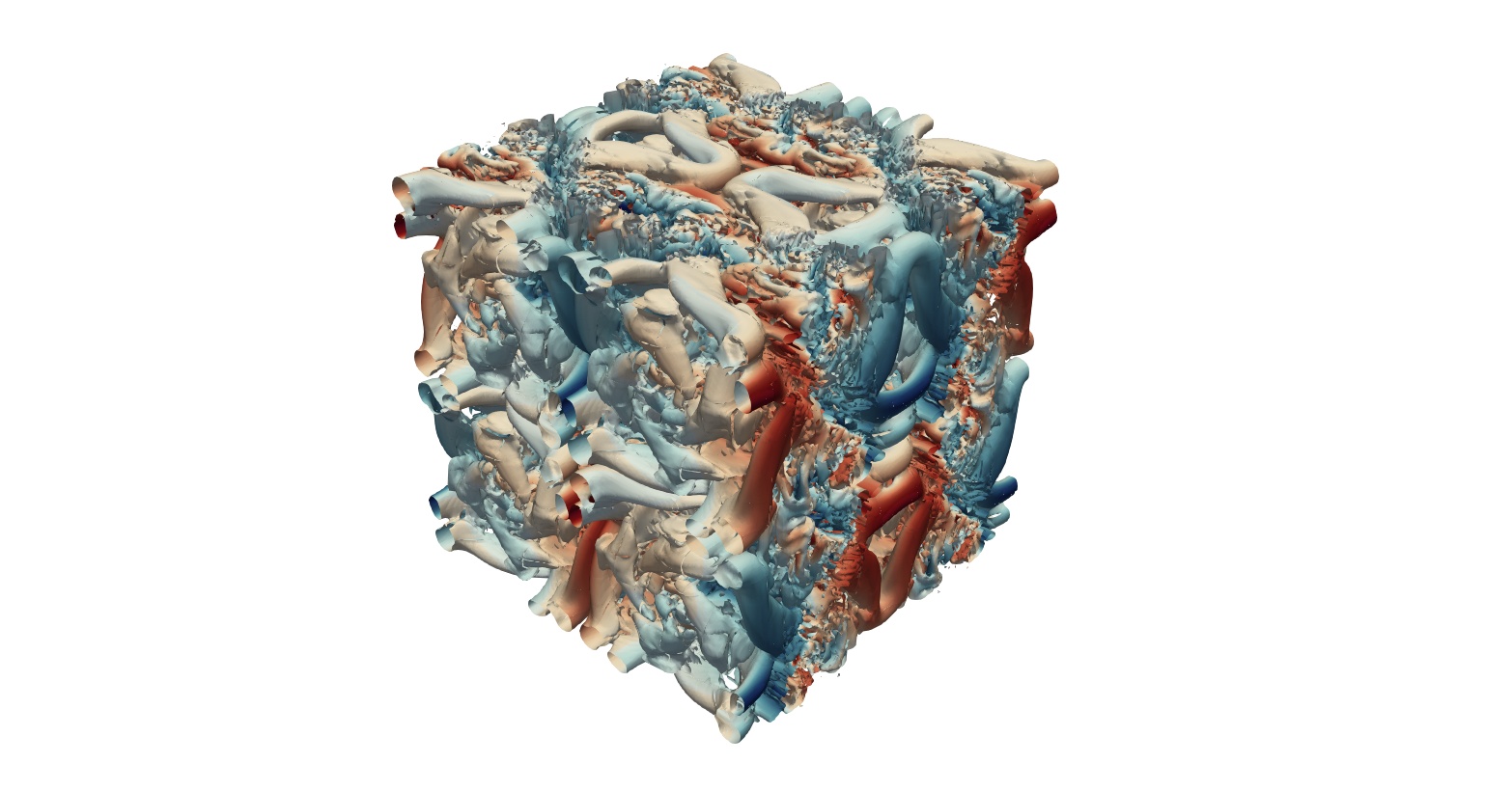
../../_images/tgv_Qcrit.jpg — Fig. 5.15 3D visualization of the Q-criterion of the Taylor–Green vortex.

5.5.2. Mesh Generation

We use a mesh with \(4\) cells per direction for the tutorial. In case you want to generate other meshes, the parameter file for HOPR is included in the tutorial directory (parameter_hopr.ini), together with the default mesh. Using \(4\) cells with a polynomial degree of \(N = 7\) results in a typical large eddy setup of \(32\) degrees of freedom (DOF) per direction.

5.5.3. Compiler Options

Depending on the dealiasing strategy used, FLEXI should be compiled either with the tgv_overintegration, tgv_split_lobatto or tgv_split_gauss preset using the following commands

cmake -B build --preset tgv_overintegration
cmake --build build

cmake -B build --preset tgv_split_lobatto
cmake --build build

or

cmake -B build --preset tgv_split_gauss
cmake --build build

respectively.

5.5.4. Simulation Parameters

The parameter file to run the simulation is supplied as parameter_flexi.ini.

5.5.4.1. Interpolation

! ============================================================ !
! INTERPOLATION
! ============================================================ !
N             = 7

The parameter N sets the degree of the solution polynomial. In this example, the solution is approximated by a polynomial of degree \(3\) in each spatial direction. This results in \((N+1)^3 = 512\) degrees of freedom for each (3D) element. In general, N can be chosen to be any integer greater or equal to \(1\), however, the discretization and the timestep calculation has not extensively been tested beyond \(N\approx 23\). Usually, for a good compromise of performance and accuracy is found for \(N\in[3,..,9]\).

5.5.4.2. Overintegration

To apply polynomial dealiasing there are the following options in FLEXI.

! ============================================================ !
! OVERINTEGRATION (ADVECTION PART ONLY)
! ============================================================ !
OverintegrationType = 0  ! 0:off
                         ! 1:cut-off filter
                         ! 2: conservative cut-off

NUnder              = 7  ! specifies effective polydeg
                         ! (modes > NUnder are thrown away)
                         ! only for types 1 and 2

In mode \(0\), polynomial dealiasing is disabled. FLEXI has two ways of doing polynomial dealiasing. In mode \(1\), a filter is applied to the time-update \(\mathcal{J}U_t\). The filter is formulated as a Galerkin projection of degree \(N\) to NUnder, the effective resolution is thus NUnder. Mode \(2\) is in principle identical to mode \(1\), but takes into account non-linear metric terms present in curved meshes. For the linear mesh in this tutorial, the result is identical. Since mode \(2\) is slightly more computational expensive, we omit it in the present tutorial.

5.5.4.3. Kinetic/Entropy Stable Formulations

An additional dealiasing technique is provided by entropy/kinetic energy stable split formulations of the DGSEM. In FLEXI, implementations either on Legendre-Gauss-Lobatto or on Legendre-Gauss integration points are available and depending on the chosen compile option. The respective split flux formulation can be specified by the following option. The most commonly used are PI, CH and SD. While the option PI [14] enables the use of a kinetic energy stable formulation, the option CH [15] provides an entropy conservative formulation of the DGSEM. Finally, the parameter choice SD yields a flux differencing form of the DGSEM which is equivalent to the standard DGSEM formulation.

! ============================================================ !
! SPLIT DG
! ============================================================ !
SplitDG             = PI ! PI: kinetic energy preserving formulation
                         ! CH: entropy conserving formulation
                         ! SD: standard DGSEM in flux differencing formulation

5.5.4.4. Riemann Solvers

Besides the inherent filtering properties of the DG operator, the only additional artificial dissipation is then provided by the Riemann solver used for the inter-cell fluxes. You can change the Riemann solver to see the effect with the following parameters:

! ============================================================ !
! Riemann
! ============================================================ !
Riemann             =  RoeEntropyFix ! Riemann solver to be used:
                                     ! LF, HLLC, Roe,
                                     ! RoeEntropyFix, HLL, HLLE, HLLEM

Attention

Be aware that from the above listed Riemann solvers, only the implementations of LF, Roe and RoeEntropyFix are compatible for the use with split flux formulations.

5.5.4.5. Sub-Grid Scale Model

To add sub-grid scale (SGS) model by Smagorinsky, set the parameter eddyViscType = 1. Here, CS is the Smagorinsky constant which is usually chosen around CS = 0.1 for isotropic turbulence (such as in the TGV).

! ============================================================ !
! LES MODEL
! ============================================================ !
eddyViscType        = 0   ! Choose LES model, 1:Smagorinsky
CS                  = 0.1 ! Smagorinsky constant
PrSGS               = 0.6 ! turbulent Prandtl number

5.5.5. Simulation and Results

We proceed by running the code with the following command.

flexi parameter_flexi.ini

If FLEXI was compiled with MPI support, it can also be run in parallel with the following command. Here, <NUM_PROCS> is an integer denoting the number of processes to be used in parallel.

mpirun -np <NUM_PROCS> flexi parameter_flexi.ini

Important

FLEXI uses an element-based domain decomposition approach for parallelization. Consequently, the minimum load per process is one grid element, i.e. do not use more processes than grid elements!

This test case generates an analysis output file named <PROJECTNAME>_TGVAnalysis.csv, which we use to examine the results. Instead of focusing on flow visualization, this tutorial centers on analyzing key quantities directly from this analysis output data. Among other interesting quantities, the analysis file contains the incompressible dissipation rate, stored in the second column of the file. This is the resolved dissipation of the gradient field, computed as the integral over the domain of the strain rate tensor norm \(S_{ij}S_{ij}\), times viscosity times \(2\). We will use this quantity in the tutorial to verify your results. You can visualize the csv file in your favored plotting tool, e.g., within ParaView using the option Line Chart View.

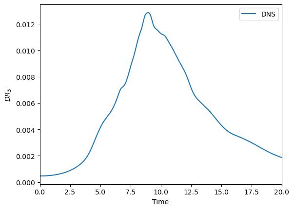
\[\mathrm{DR}_S = \frac{2 \mu}{\rho_0 \lVert \Omega \rVert } \int_\Omega S_{ij} S_{ij} ~ d\mathbf{x}\]

../../_images/tgv_dns.jpg — Fig. 5.16 Incompressible dissipation rate of the Taylor–Green vortex over time.

5.5.5.1. Part I: Crashing Simulation

First, we run FLEXI without any kind of dealiasing technique. For this, use the FLEXI version compiled with the preset tgv_overintegration. We will find that the code crashes, once scale production becomes relevant. The same holds for the split form DGSEM if used with the SD split flux and the preset tgv_split_lobatto or tgv_split_lobatto- You can compare your result to the crash_no_dealiasing.csv file in the tutorial folder.

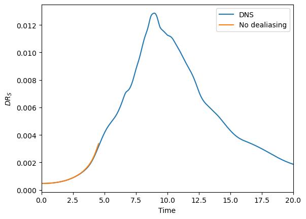
../../_images/tgv_nodealiasing.jpg — Fig. 5.17 Incompressible dissipation rate of the Taylor–Green vortex over time without any dealiasing technique.

5.5.5.2. Part II: Overintegration

We now use overintegration by changing the respective settings in the parameter_flexi.ini file as described above. Set OverintegrationType = 1 and specify N = 11 and NUnder = 7. You can compare your result to the les_overintegration.csv file in the tutorial folder.

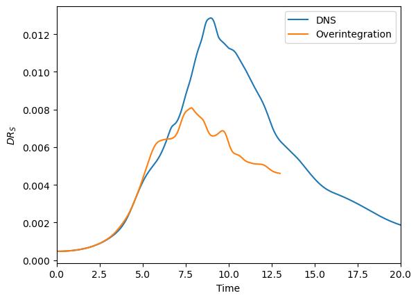
../../_images/tgv_overintegration.jpg — Fig. 5.18 Incompressible dissipation rate of the Taylor–Green vortex over time with overintegration.

5.5.5.3. Part III: Split Formulation

We now use the split DGSEM formulation as a dealiasing technique. Please be aware to use FLEXI either compiled with the preset tgv_split_lobatto or tgv_split_gauss. Set SplitDG = PI and specify N = 7. Don’t forget to switch off overintegration. You can compare your result to the les_split.csv file in the tutorial folder.

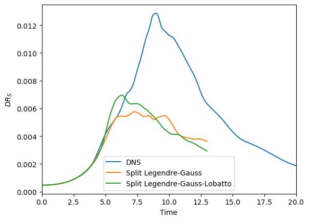
../../_images/tgv_split.jpg — Fig. 5.19 Incompressible dissipation rate of the Taylor–Green vortex over time with a kinetic energy stable formulation.

5.5.5.4. Part VI: Explicit LES model

To see the effect of adding explicit eddy viscosity, we activate the LES model (Smagorinsky) as described above via eddyViscType = 1. To obtain the reference result in les_smago.csv, set CS = 0.1. Don’t forget to switch back to the compiler preset tgv_overintegration and deactivate overintegration OverintegrationType = 0. Use a polynomial degree of N=7.

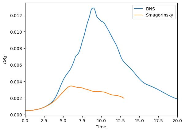
../../_images/tgv_smago.jpg — Fig. 5.20 Incompressible dissipation rate of the Taylor–Green vortex over time with the Smagorinsky model as a sub grid scale model.

5.5.5.5. Part V: Have Fun!

Feel free to play around with the effect of the constant in the Smagorinsky model or compare the different dealiasing techniques with respect to accuracy or compute time. Most important, have fun with FLEXI.