5.1. Linear Scalar Advection-Diffusion Equation

The three-dimensional linear scalar advection-diffusion (LinAdvDiff) equation implemented in FLEXI provides a simple and computationally efficient system of equations for testing and feature development:

\[\frac{\partial \Phi}{\partial t} + \nabla \cdot (\mathbf{u}\Phi) = d \nabla^2 \Phi\]

Here, a scalar solution \(\Phi\) is advected with a constant three-dimensional velocity \(\mathbf{u}\) and experiences diffusion with a constant scalar diffusion coefficient \(d\). This equation is especially useful for evaluating the basic properties of the DG operator, which we will explore in this tutorial. The tutorial is located at tutorials/linadv.

5.1.1. Theoretical Background

The dispersion and dissipation properties of the DGSEM operator can be analyzed [17] by examining the evolution of solutions for the one-dimensional linear scalar advection equation for a specific initial wave number in a simplified setup without physical dissipation (\(d=0\)). A detailed discussion can be found in the cited paper; here, only a short summary is presented.

Under these preceding conditions, the equation reduces to

\[\frac{\partial \Phi}{\partial t} + u\frac{\partial \Phi}{\partial x}=0\]

and we consider a wave-like analytical solution on an infinite domain,

\[\Phi(x,t)=e^{i(kx-\omega t)}\]

where \(u\) is a constant scalar transport velocity, \(\omega = ku\) the angular frequency, and \(k\) the wavenumber. Assuming a uniform mesh with mesh size \(\Delta x\), we seek numerical solutions of the form

\[\mathbf{\Phi}^l = \hat{\mathbf{\Phi}} e^{i(kl\Delta x-\omega t)}\]

where \(\mathbf{\Phi}^l\) is a vector containing the degrees of freedom within cell \(l\), and \(\hat{\mathbf{\Phi}}\) is a complex amplitude vector, both of size \(N+1\). Focusing on the semi-discrete system (only spatially discretized), we can write the system in matrix notation within a single element, yielding an algebraic eigenvalue problem

\[\underline{\underline{A}} \hat{\mathbf{\Phi}} = \Omega \hat{\mathbf{\Phi}},\]

with \(\Omega = \frac{\omega \Delta x}{a}\). The matrix \(\underline{\underline{A}}\) represents the spatial discretization and is a function of the non-dimensional wavenumber \(K = k \Delta x\).

Examining the solutions to this eigenvalue problem reveals relationships for the dissipation and dispersion behavior inherent to the (spatial) numerical scheme for different wavenumbers. In Fig. 5.1, we plot these relationships as functions of the polynomial degree \(N\), using DGSEM with Gauss nodes for the so-called physical mode. This mode is associated with the eigenvalue that follows the exact dispersion relation for the largest range of wavenumbers and also has the biggest influence on the overall numerical solution, at least for rather well-resolved waves.

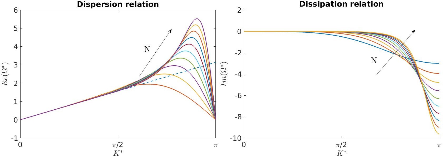
Fig. 5.1 Dispersion and dissipation relationship for \(N=\{1,\ldots,10\}\) over the modified wavenumber \(K^*\). For the dispersion, the dashed line gives the exact relation.

The quantities are normalized by the number of grid points, such that \(K^* = \frac{K}{N+1}\) and \(\Omega^* = \frac{\Omega}{N+1}\), to give a fair comparison between different polynomial degrees. This means that if \(K^* = \pi\), we have two points per wavelength which is the theoretical minimum required to resolve a wave according to the Nyquist theorem, while a normalized wavenumber of \(0\) corresponds to a constant solution.

As seen in the plot, the dissipation properties of higher-order approximations are significantly improved over those of low-order schemes, as they can preserve higher-frequency waves without significant dissipation. However, there is a sharp increase in dissipation error at the high modes associated with higher-order approximations, which is one of the reasons for scaling down the timestep for larger values of \(N\).

We will now demonstrate these properties through numerical experiments using the linear scalar advection equation.

5.1.2. Build Configuration

In order to use the LinAdvDiff equations, the equation system must be specified during the configuration by setting EQNSYSNAME=linearscalaradvection. Since we do not consider diffusion in this tutorial, either turn off the parabolic terms through the build option FLEXI_PARABOLIC=OFF or simply specify a zero diffusion coefficient in the parameter file, DiffC=0. The required options are set automatically by compiling FLEXI with the linadv preset using the following commands.

cmake -B build --preset linadv
cmake --build build

5.1.3. Mesh Generation

We want to perform numerical experiments by solving the one-dimensional linear scalar advection equation. We initialize the simulation with a single wave with a specific angular frequency and observe the behavior of this wave as it evolves, depending on the normalized, non-dimensional wavenumber \(K^*\) and the polynomial degree \(N\). Since the analysis in the previous section was based on an infinite domain, the computational domain needs to be large enough to neglect influences from the boundaries. Although periodic boundary conditions could be used as an alternative, this would restrict the choice of wavelengths since they have to fit in the domain and could also adversely affect the stability of the time discretization. Therefore, we opt for an enlarged domain setup and focus on the evolution of the wave in a single element at the center of the domain.

For this tutorial, we create a (quasi-)one-dimensional, equidistant grid by discretizing the interval \(x \in [-61,61]\) with 61 elements, resulting in \(\Delta x = 2\), which matches the reference element size. To achieve a (quasi-)one-dimensional simulation, we impose periodic boundary conditions in \(y\) and \(z\) direction. The boundary conditions in the \(x\)-direction are less critical due to the large extent of the domain, so we apply a simple Dirichlet-type boundary conditions (BC type 2) with the analytical wave function as the boundary state. This can be achieved by setting the BC_STATE, which means that the initialization function will be used instead of a separate function. Recall that for the LinAdv case, information propagates with the velocity \(u\). Thus, if the boundaries are a distance \(L\) away from the cell of interest, solutions can be computed up to time \(t = \frac{L}{u}\) without any influence of the boundary conditions.

In the tutorial directory, we provide the necessary mesh file, CART_1D_mesh.h5, along with a parameter file for HOPR to generate this mesh. You can recreate the mesh by running the following command.

hopr parameter_hopr.ini

5.1.4. Simulation Parameters

The parameter file to run the simulation is supplied as parameter_flexi.ini. The parameters specific to the LinAdvDiff equation system can be found in the EQUATION section of the file.

! ============================================================ !
! EQUATION
! ============================================================ !
AdvVel        = (/1.,0.,0./)
DiffC         = 0.

The parameter AdvVel sets the advection velocity in all three spatial directions. In our one-dimensional simulation, only the first velocity component is non-zero. We set the diffusion coefficient DiffC to zero to eliminate physical diffusion, although this is not strictly necessary since the parabolic terms have already been excluded via the build configuration.

The initial condition is derived from the earlier analysis outlined above, with the exact solution given by

\[\Phi(x,t) = e^{i(kx - \omega t)}.\]

The amplitude of the wave is given by the real part of this complex expression

\[A(x,t) = cos(kx-\omega t).\]

This function is implemented as ExactFunc in the LinAdvDiff equation system and is called by specifying

IniExactFunc  = 6

in the parameter file. This requires definition of the angular frequency \(\omega\), since the wavenumber is given by \(k=\frac{\omega}{u}\), so

OmegaRef      = 2.

Note that the ExactFunc function implements the advection velocity and diffusion coefficient as fixed default values, which override the parameters specified in the parameter file. To focus on the behavior of the spatial discretization while minimizing the error from time discretization, we set the CFL number to a small value

CFLscale      = 0.1

Given that this tutorial involves a quick computation, we can utilize the visualization routines during runtime, eliminating the need for post-processing with the posti_visu tool. This is accomplished by enabling the vtu output format. With this configuration, the visualization routines are called whenever the analysis routines are executed, with NVisu defining the polynomial degree of the output basis. Since we do not specify Analyze_dt in the parameter file, the analysis routines will only be invoked at the beginning and end of the simulation.

outputFormat  = 3
NVisu         = 30

5.1.5. Simulation and Results

We start with simulating a well-resolved wave using a moderate polynomial degree of \(N = 4\), which is already configured in the parameter file. For a modified wavenumber of \(K^* = \frac{1}{4}\pi\), the dissipation and dispersion relations indicate that we can expect very small errors. Using the relations above, the corresponding angular frequency \(\omega\) can be calculated as

\[\omega = \frac{K^* (N+1)}{\Delta x} u.\]

Hence, we adjust the frequency in the parameter file to

OmegaRef      = 1.96349540849

All other parameters can remain unchanged. The simulation will run until \(t=5\) and is started by executing

flexi parameter_flexi.ini

After the simulation has completed, we can examine the results by opening the file LinAdvCosineWave_Solution_0000005.000000000.vtu with ParaView. As noted earlier, we are only interested in the central element within \(x \in [-1, 1]\), so we can clip everything else. Moreover, given that we are performing a one-dimensional simulation, we can extract the solution along the \(x\)-axis by creating a simple line plot. To see how dispersion and dissipation introduced by the numerics influence our results, we will also overlay the analytical solution introduced above. The result is depicted in figure Fig. 5.2 and shows very little deviation from the analytical solution, as expected, since we are analyzing a well-resolved wave with a low value for \(K^*\).

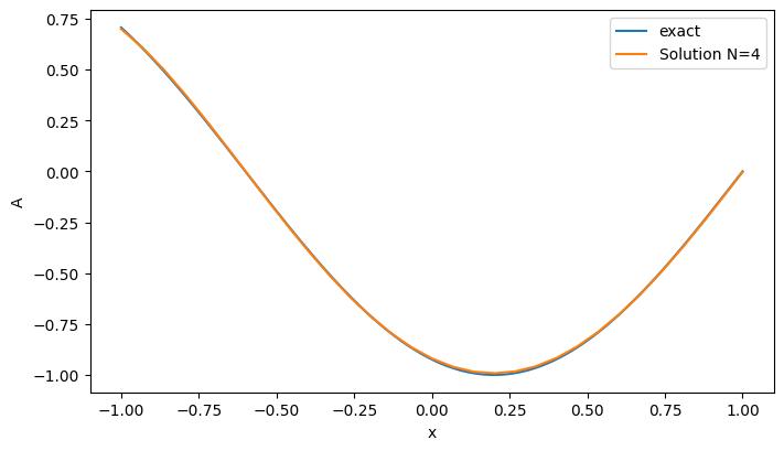
Fig. 5.2 Result for a well-resolved wave with \(K^*=\frac{1}{4}\pi\) at \(t=5\) for \(N=4\), in comparison with the exact wave transport.

Of course, it is much more interesting to examine the behavior of waves that are not well-resolved and how the polynomial degree affects their dynamics. To explore this, we run four simulations with polynomial degrees ranging from \(2\) to \(11\) and setting the normalized wavenumber to \(K^* = 1.6\). Table 5.1 gives an overview of the polynomial degrees and the resulting angular frequencies.

Table 5.1 Angular frequencies needed to attain \(K^*=1.6\).

N	OmegaRef
2	2.4
4	4.0
6	5.6
11	9.6

Next, we will run these four simulations by adjusting the values for N and omegaRef in the parameter file prior to each run. Remember to give each simulation a unique ProjectName to prevent overwriting the results. Additionally, ensure that NVisu is set to at least three times the value of \(N\) to obtain a meaningful visualization. As we already set NVisu=30, simply leave this value unchanged.

The results at \(t=5\), along with the analytical solutions, are shown in Fig. 5.3. Since our comparison uses a constant normalized wavenumber, the actual frequency of the wave increases with the polynomial degree. For \(N=2\) (which should not be considered high-order), we observe both significant dissipation, with an amplitude drop of about \(85\%\), and notable dispersion, that is variations in angular frequency and phase angle. At \(N=4\) (which is at the lower end of what can be considered high-order) there are already some improvements. The amplitude drop is reduced to around \(65\%\), although a phase shift remains clearly visible. This trend continues at higher polynomial degrees. For the highest value of \(N\) tested here, we observe only small deviations in the phase angle and the amplitude. These results show how higher-order schemes are able to effectively capture waves with fewer points per wavelength compared to lower-order approximations. This is one of the central aspects why we use such schemes.

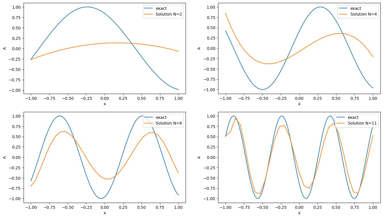
Fig. 5.3 Result for a under-resolved wave with \(K^*=1.6\) at \(t=5\) for \(N=2\) (top left), \(N=4\) (top right), \(N=6\) (bottom left) and \(N=11\) (bottom right).