Preprint – 22.06.2023
Towards Exascale CFD Simulations Using the Discontinuous Galerkin Solver FLEXI
We have a new preprint out that shows some steps taken towards exascale computing with FLEXI. Enjoy!!
Abstract
Abstract Modern high-order discretizations bear considerable potential for the exascale era due to their high fidelity and the high, local computational load that allows for computational efficiency in massively parallel simulations. To this end, the discontinuous Galerkin (DG) framework FLEXI was selected to demonstrate exascale readiness within the Center of Excellence for Exascale CFD (CEEC) by simulating shock buffet on a three-dimensional wing segment at transsonic flight conditions.
This paper summarizes the recent progress made to enable the simulation of this challenging exascale problem. For this, it is first demonstrated that FLEXI scales excellently to over 500 000 CPU cores on HAWK at the HLRS. To tackle the considerable resolution requirements near the wall, a novel wall model is proposed that takes compressibility effects into account and yields decent results for the simulation of a NACA 64A-110 airfoil. To address the shocks in the domain, a finite-volume-based shock capturing method was implemented in FLEXI, which is validated here using the simulation of a linear compressor cascade at supersonic flow conditions, where the method is demonstrated to yield efficient, robust and accurate results. Lastly, we present the TensorFlow-Fortran-Binding (TFFB) as an easy-to-use library to deploy trained machine learning models in Fortran solvers such as FLEXI.
To the full Paper
http://dx.doi.org/10.48550/arXiv.2306.12891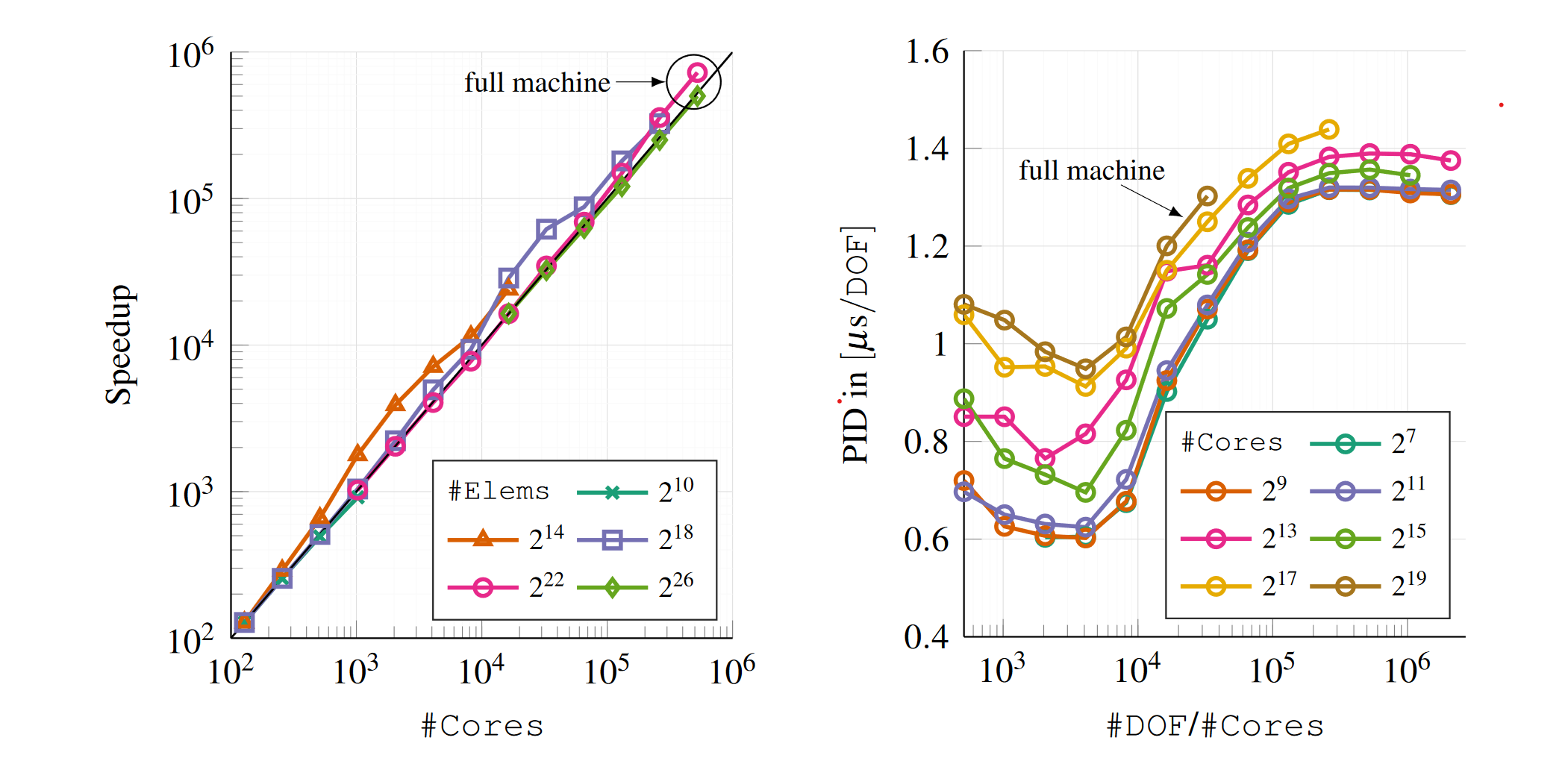
Scaling of FLEXI on HAWK. Left: Strong scaling results as speedup formeshes comprising different number of elements. The ideal speedup is indicated inblack. Right: PID over the specific load per core for different numbers of computenodes. Only the mean is shown in both cases for the sake of clarity.
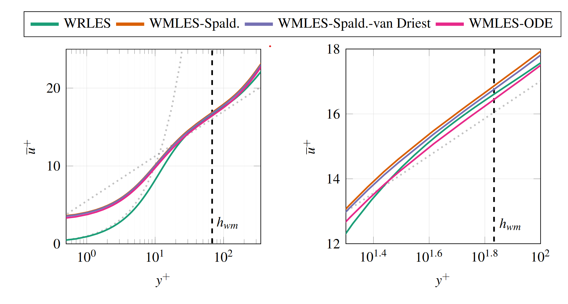
Comparison of the mean velocity profile of a NACA 64A-110 airfoil on thepressure side at x = 0.5c with a detailed view of the log layer on the right. The linear behavior in the viscous sub-layer and the log-law are depicted by dotted gray lines and the wall model exchange location hwm is indicated by a dashed line.
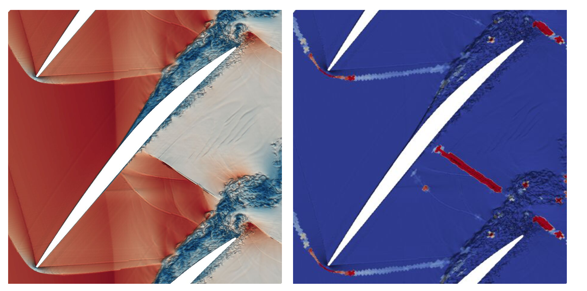
Left: Instantaneous flow field around the NASA Rotor 37 blade colored bythe Mach number. High Mach numbers, Ma = 1.7, are highlighted in red and lowones in blue. Right: Values of the blending coefficient. Low values, αFV = 0, arecolored in blue and high values, αFV = 0.7, in red.